Human mobility patterns in different communities: a mobile phone data-based social network approach

Figures & data

Figure 1. Spatial distribution of mobile base towers (dots) and associated Thiessen polygons. © [OpenStreetmap and contributors]. (The base map is obtained from OpenStreetmap, following the creative commons-share alike license. http://creativecommons.org/licenses/by-sa/2.0/)

Figure 2. Basic features of mobile social network. (A) Complementary cumulative distribution of degree; (B) Relationship of giant component’s size versus call frequency threshold. The giant component of the original network contains more than 96% of the nodes.

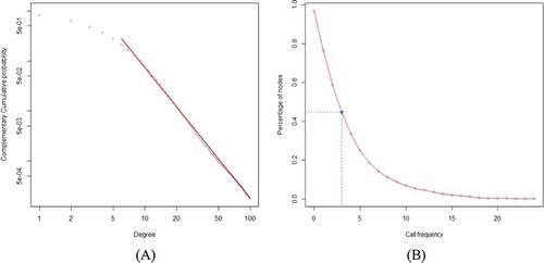
Figure 3. Spatial distributions of single-centred communities. Figure A, B and C show the small single-centred communities, while D, E and F show the large single-centred distributions.

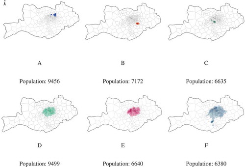
Figure 4. Spatial distributions of dual-centred communities.

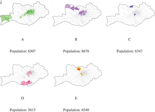
Figure 5. Spatial distributions of zonal communities.

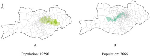
Figure 6. The angle distribution of different communities. For simplicity, we only choose two communities of each pattern to display their angle distributions. The community identifier in the legend of each pattern corresponds to Figures 3, 4 and 5.

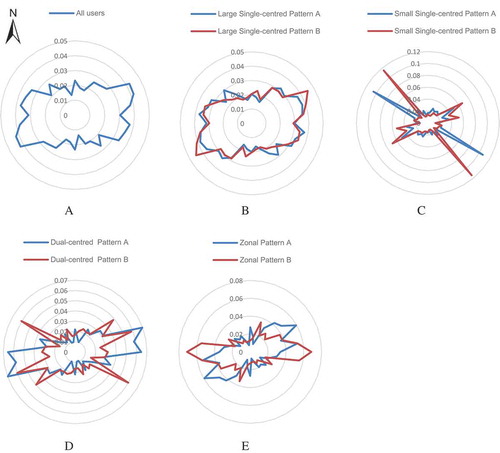
Figure 7. ROG distribution of different community patterns. The order of the proportion of users with ROG smaller than 3 km is small single-centred, large single-centred, zonal and dual-centred. The majority (more than 60%) of users in small single-centred communities have ROG less than 3 km. The proportion of users in dual-centred communities is the largest to have ROG larger than 3 km. The ROG of more than 20% of users in dual-centred communities are larger than 8 km.

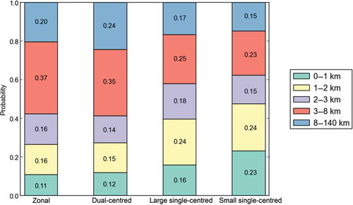
Figure 8. Illustration of how trajectories of home–work-separate persons in two centres are extracted. For a dual-centred community, Region #1 and Region #2 cover areas of two centres located in the urban district and suburb, respectively. We name Region #1 as ‘urban centre’ and Region #2 as ‘suburban centre’. Both individuals A and B are home–work-separate persons in suburban centre, while individual C is a home–work-separate person in urban centre. Trajectory distribution of urban residents is generated by the set of trajectories of persons such as C, and trajectory distribution of suburban residents is created by the set of trajectories of persons like A and B.

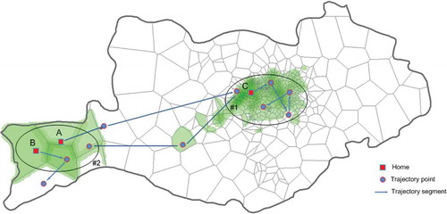
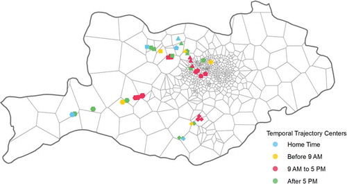
Figure 9. Trajectory distributions of urban residents and suburban residents for the five dual-centred communities. The left and right columns illustrate trajectory distributions of dual-centred community residents who live in urban and suburban area, respectively. Each row in sequence corresponds to a community in Figure 4 in the alphabetical order. Trajectories of individuals living in urban centre are distributed generally around the urban district while trajectories of persons in suburbs are distributed in both urban district and suburbs.

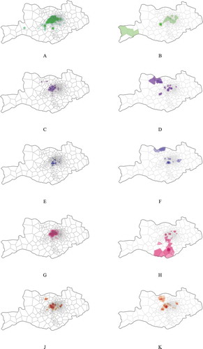
Figure 10. Temporal trajectory centres of bridge residents in each dual-centred community (represented by different symbols). Only the centre points at odd hours are shown for clarity. Bridge residents are referred to residents who live in suburban centres while working in urban centres. The temporal trajectory centres demonstrate that the forming of dual-centred communities is strongly influenced by the commuting behaviours of those bridge residents.