
Figures & data
Figure 1. Framework of the proposed method.
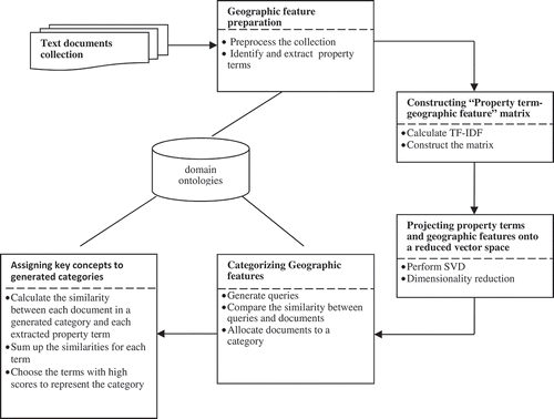
Table 1. An example: property term–geographic feature matrix.
Figure 2. An example: the produced three matrices, U, S and V, by SVD with dimension reduction (k = 2).
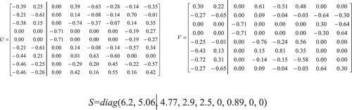
Table 2. The predefined categories generated based on vegetation community types in the state of New Mexico.
Figure 3. Mountains’ locations and vegetation community types in the state of New Mexico. Each point represents the centre location of a mountain.
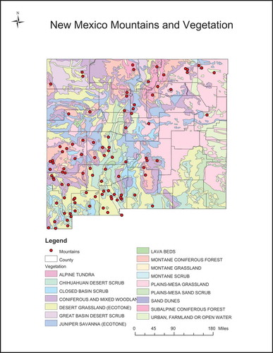
Figure 4. F1 scores and threshold p.
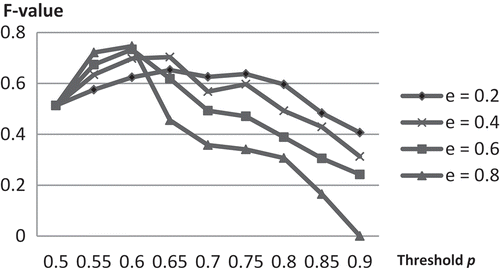
Figure 5. Reduced dimension k and threshold p.
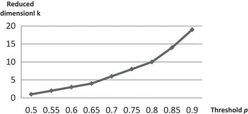
Figure 6. Precision, recall and F1 score values with threshold e (p = 0.6).
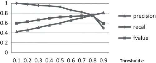
Table 3. The categorization results (p = 0.6, e = 0.8).
Figure 7. Categorization results: a map of mountains for the predefined and generated category ‘coniferous and mixed woodland’ (p = 0.6, e = 0.8).
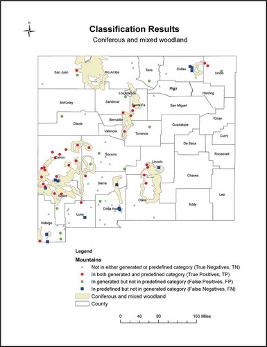
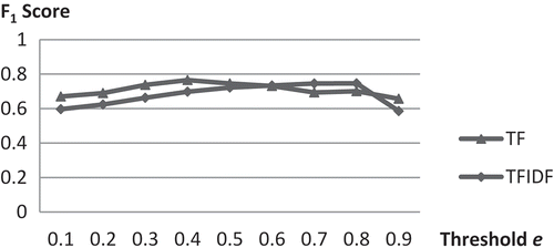
Figure 8. Comparison of TF and TF-IDF with threshold e.
Appendix A. Comparison of the TF-IDF and TF in terms of key concept identification (p2 = 0.8).