Figures & data
Figure 1. Generation of the cross track antenna using repeated flights.
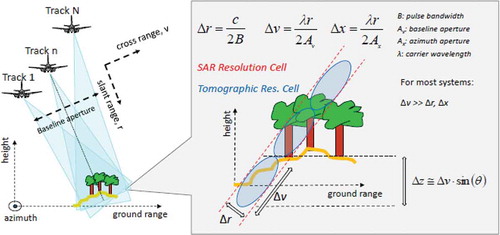
Figure 2. The Remingstorp forest (left) and at right a cartoon representing the components of a cross range resolution cell: the double bounce (down) and the canopy reflection (up) are clearly indicated.
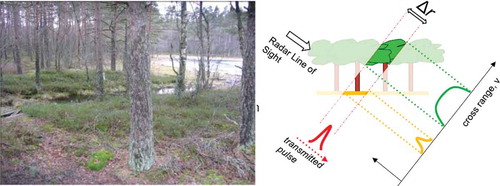
Figure 3. A vertical section from the Capon tomographical spectra of a transect of the Remningstorp forest; channels HH and HV.
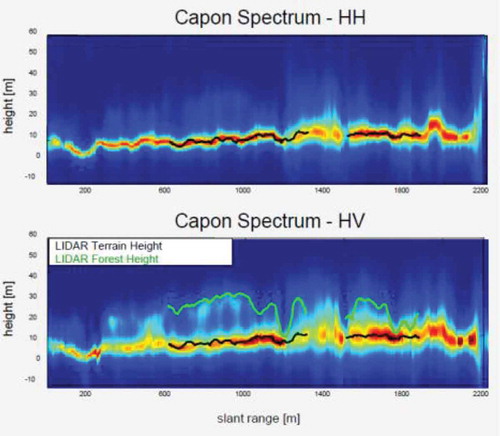
Figure 4. Ground (down) and canopy (up) heights.
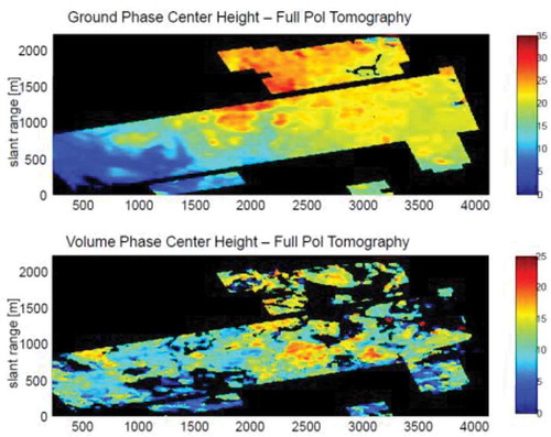
Figure 5. The Guyaflux tower in Paracou (French Guyana) and its trace through the 4 tomographic layers.
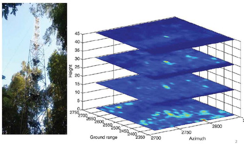
Figure 6. The reflectivities of the 4 layers in French Guyana.
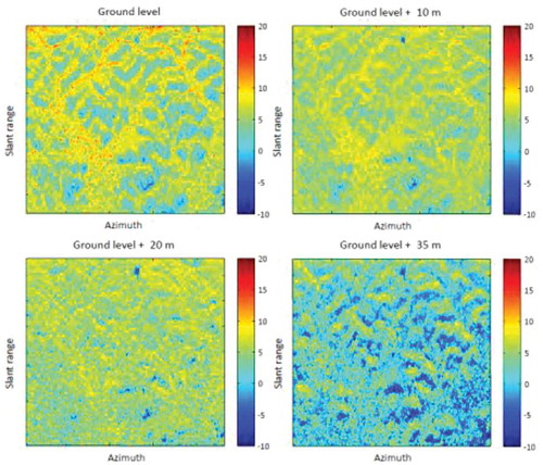
Figure 7. Relation between above ground biomass and reflectivity of each tomographic layer.
Figure 8. The Tropiscat antenna on the Guyaflux tower, and the tomographic views in the 4 polarimetric channels.
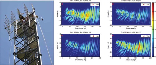
Figure 9. 17 days coherence of the tomographic data shown in Figure 8.
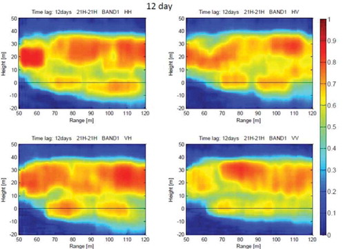
Figure 10. Simulation of the SAOCOM CS results: LIDAR (top) and tomographic (bottom) vegetation heights.
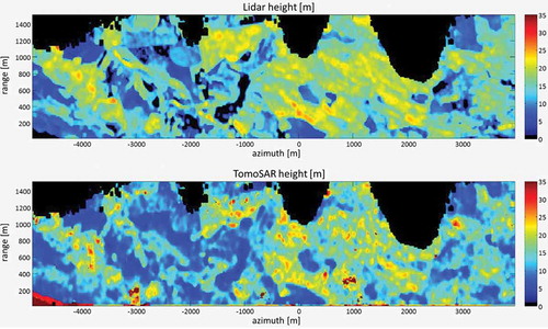
Figure 11. Simulation of the SAOCOM CS results: a transect in the three polarimetric channels.
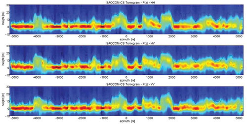
Figure 12. The Mittelbergferner glacier (Austrian Alps).
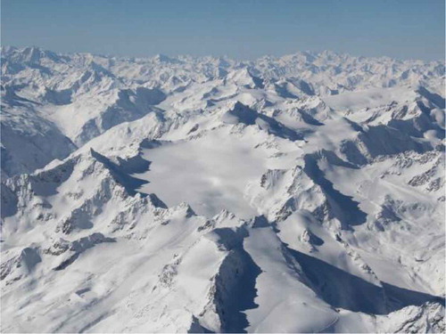
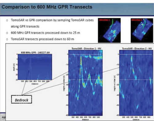
Figure 13. Tomographic results of the two airborne passes (right) compared with the 600MHz GPR data (left).