Figures & data
Figure 1. Map of the study area with two selected study reaches, namely the Upper Reach (UR) and Lower Reach (LR) in southeastern Louisiana; River Miles are also included in this map.
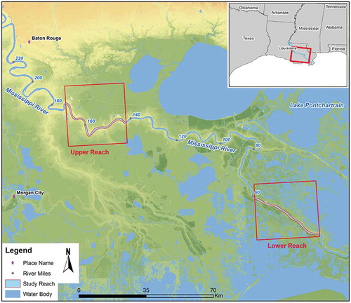
Table 1. Summary of selected studies with corresponding interpolation methods in generating bathymetry. (A) summarizes the studies related to river channels (except Mississippi River); whereas (B) compiles the studies related to other waterbodies (i.e., coastal and lake). The studies in Mississippi River and its tributaries, especially LMR (Lowermost Mississippi River) are organized in (C).
Figure 2. The bathymetric cross-sections in UR (a) and LR (b) reaches (see for the locations). Each cross-section contains ~20 to 30 soundings labelled in red dots. The numbers represent River Miles. Note that although the original hydrographic surveys were labelled in English unit (mile, feet), all the calculated results are converted into metric system.
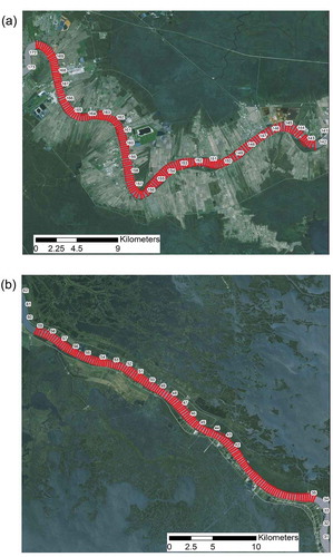
Figure 3. An example of coordinate transformation from Cartesian (x, y) coordinate system (a) into channel-centred (s, n) coordinate system from a selected portion in study reaches. The channel centreline is shown in (a), which would be transformed to reference line with n = 0 in n-axis in (b). The soundings with different colour represent the bed elevation.
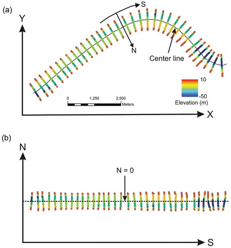
Figure 4. IDW interpolation methods (a) with sampled points P1 to P5 and unsampled point P in the centre, circular with dashed line represent its search neighbourhood, note that P5 is excluded in the search circle. Nevertheless, (b) shows elliptical search neighbourhood for EIDW algorithm (major axis = a, minor axis = b), and P5 is included in this case. (Modified from Merwade, Maidment, and Goff Citation2006).
Table 2. Parameters used in the different spatial interpolation methods in both of UR (A) and LR (B) regions.
Figure 5. Trend analysis for the cross-sectional data in UR reach (A) and LR region (B) in 3D frames. Both figures were created by using ArcGIS. The green lines represent x, y, z dimensions. Each black dot symbolizes the bathymetric measurement; and -axis display vertical elevation. Note that in channel-centred (s, n) coordinates, red and blue lines represent the trend lines for x-direction (s-axis) and y-direction (n-axis), respectively.
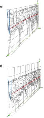
Table 3. Summary of the statistical results for different interpolation methods by using leave-one-out cross-validation in UR (A) and LR (B) reaches.
Figure 6. The experimental semivariograms and semivariogram maps (the ellipse with different colors) in UR (A) and LR (B) areas for consideration of OKA algorithm. Clear anisotropy could be found with main direction at degree of 180 (A) and 90 (B) labeled with red dashed lines. Both experimental semivariograms were created by considering anisotropy and the parameter in .
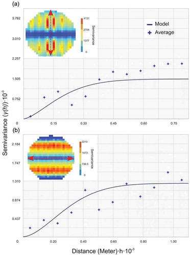
Figure 7. The interpolated bathymetric surface in UR regions by using different interpolation methods of OK (a), OKA (b), UK(c), IDW (d), EIDW (e), TPS (f) and LPI (g). The square with black line indicates the location of (a,c).
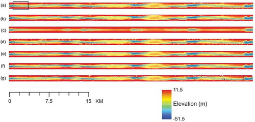
Figure 8. The interpolated bathymetric surface in LR region, with similar order of interpolation methods from . The square with black line represents the location of (b,d).
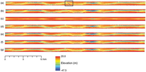
Figure 9. Different scatter-plots between observed and estimated elevation values by using interpolators of OK ((a) in UR region, (b) in LR region) and TPS ((c) in UR reach and (d) in LR reach). Different colour represent different rank ((a) to (d)) with absolute error range (A < 5 m, B = 5–10 m, C = 10–15 m, D > 15 m).
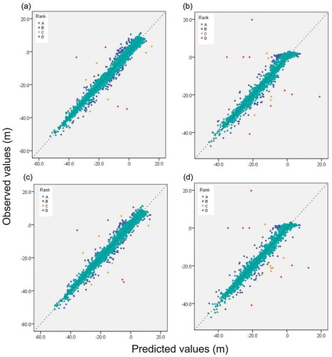
Table 4. Summary of the statistical results for different interpolation methods by using split-sample validation in UR (A) and LR (B) reaches.
Figure 10. Spatial distribution of error (points with different colours) in different selected area. The error points in plot (a) and (c) are located in UR region (as indicated) and generated by using the OKA (a) and TPS (c) interpolators; whereas error points in plot (b) and (d) are located in UR region (as indicated) and generated by using OKA (B) and TPS (d) interpolators. The background elevations are trimmed from the interpolated surfaces in and with coincided locations and interpolators. Different colours represent different error ranks as well as the ranges in . Similar distribution patterns of huge errors (circled in black dashed lines) are found in the same area with different interpolators.
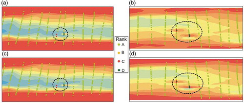
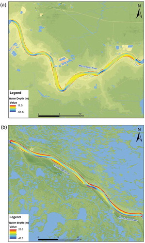
Figure 11. Bathymetric maps of UR region (a) and LR region (b) by using the TPS interpolator in Cartesian (x, y) coordinate system. The spatial resolution of these DEMs are at 10 m × 10 m.