Figures & data
Figure 1. Digital bathymetric model of the Western Mediterranean Sea. The red rectangle delimits the area under study. Source: Imagery reproduced from GEBCO_2019 Grid
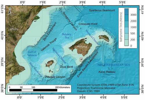
Figure 2. (Left) Cabrera Bathymetric Terrain Model. In red, location of the study area, showing linear rocky outcrops in ENE-WSW direction. (Bottom top) DBM of the continental shelf of Mallorca island. (Bottom right) Zoomed shaded relief image of the SE corner of the Cabrera continental shelf, illustrating the extent of the seabed ridges
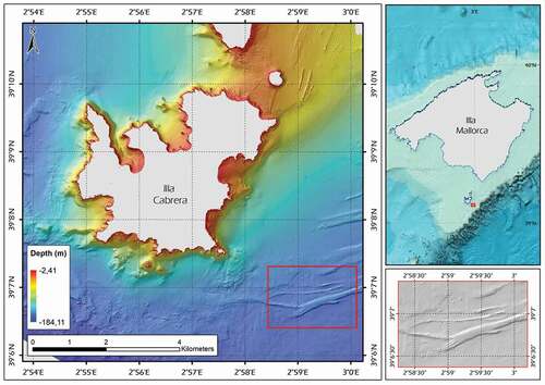
Figure 3. (a) Shipeck dredge. (b) Sediment sample. Source: OAPN
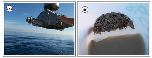
Figure 4. Overview of ground-truthing stations superimposed on bathymetry hill shade with a contour interval of 1 m. Sediment samples (orange circles) and camera stations (green triangles)’ location at the study area
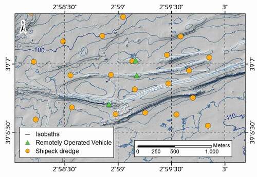
Figure 5. Flow diagram of the processing steps, starting from the multibeam echosounder acquisition (A), followed by the original depth soundings and backscatter values stage (B), showing representative examples of cleaned and validated data (C) per feature extraction method and resulting in the corresponding features for bathymetry (D) and backscatter (E).
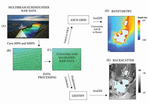
Figure 6. (a) Detailed 1-meter resolution multibeam shaded relief bathymetry (hillshade 6x vertical exaggeration) in the Cabrera southeast continental shelf. Colour scheme range for depth values is in meters, from red (lowest) to blue (highest). (b) Backscatter (300 KHz) intensity in the Cabrera southeast continental shelf. Yellow zones indicate a strong backscatter signal and green zones indicate weaker backscatter signals. Backscatter intensity is in decibels
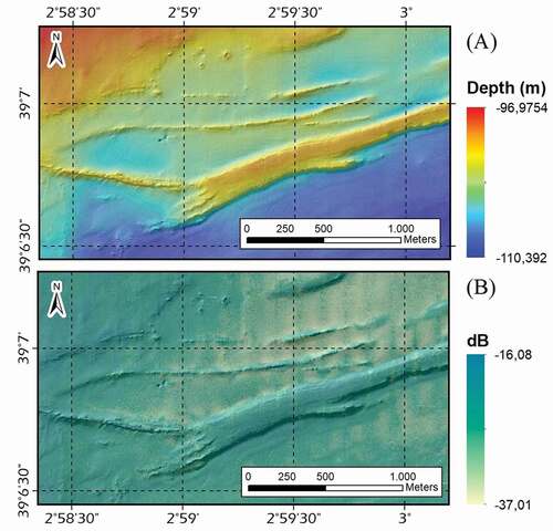
Figure 7. Predicted seafloor substrate distribution extracted from backscatter intensity. Granulometric analysis determined on sediment samples. Spatial variability in the percentages of mud, sand and gravel contents in surface sediment. The pies represent the quantification of textural composition. G: Gravel; GS: Gravelly Sand; MCS: Medium Coarse Sand; CS: Coarse Sand; S: Sand; SM: Sandy Mud; MS: Muddy Sand; M: Mud
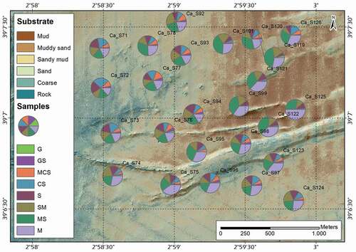
Figure 8. Detail of remotely operated vehicle images. (a) Ca_F72. Rocky outcrops (b) Ca_F73. Presence of equinodermus (Echinus Sp.) (c) Ca_F73. Linear rocky outcrops with presence of three-tailed fish bank (Anthias anthias) (d) Ca_F74. Axinella sp. (e) Ca_F74. (Palinurus elephas) (F) ROV locations
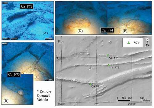
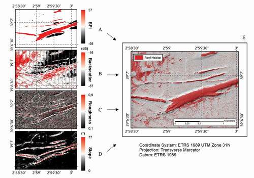
Figure 9. (Left) Spatial distribution of values of the four environmental variables used to build habitat suitability models through the bathymetric analysis. (a) Slope gradient (b) Roughness Index (c) Fine Bathymetric Position Index (d) Broad Bathymetric Position Index (BPI). (Right) Two specific subareas, four in isolated outcrops (A1, B1, C1, D1) and four in elongated outcrops (A2, B2, C2, D2), are indicated by a black square in the main map
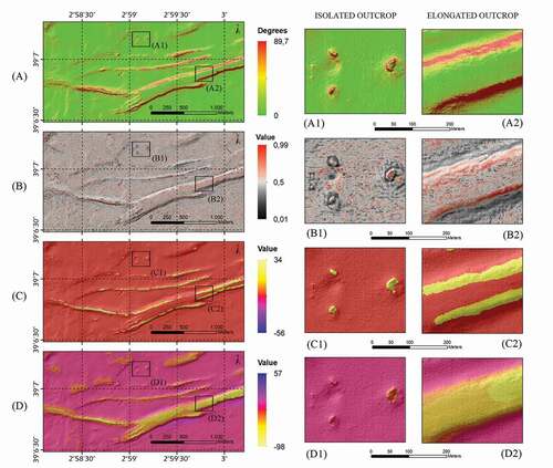
Figure 10. Example of mapping results showing a potential habitat distribution map for reefs overlaid on a hillshade image of the bathymetry. The red zones represent terrain with certain environmental conditions for the location of 1170 reef habitat. (a) Bathymetric Position Index (b) Backscatter intensity (c) Roughness Index (d) Slope gradient (e) Final reef habitat model with the combination of all these variables. Only rocky outcrops that were occupied by potential habitat reef areas are shown