Revealing intra-urban hierarchical spatial structure through representation learning by combining road network abstraction model and taxi trajectory data

Figures & data

Figure 1. The flowchart of the proposed representation learning framework for extracting hierarchical intra-urban spatial structure.

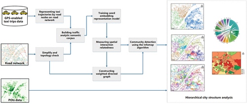
Figure 2. An example of mapping a raw taxi route to intersection nodes sequence along the road network.

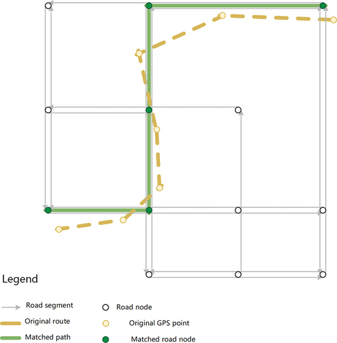
Figure 3. Our study area in Wuhan, which covers the downtown area of this city (within the third ring road). (a) Administrative districts of Wuhan city; (b) Satellite remote sensing image of the study area. The bottom images show examples of diverse landscapes: (1) industrial area, (2) residential area, (3) commercial area and (4) educational area.

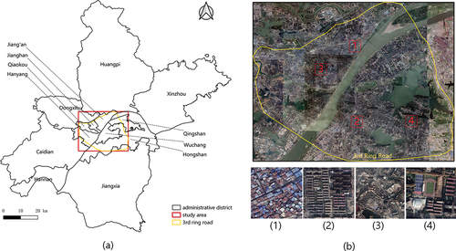
Figure 4. Data schema of the road network in the study area. (a) road segments and (b) road nodes.

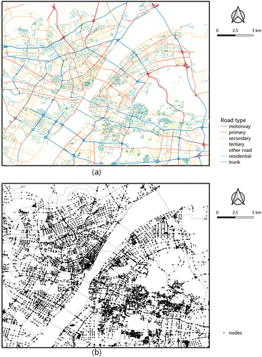
Figure 5. (a) kernel density estimation of pois (unit: count per km²); (b) spatial distribution of POIs near Jianghan road, a famous commercial area within the downtown of Wuhan. Note that different colours indicate types of POIs.

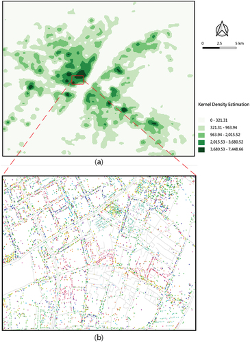
Figure 6. Relationship between the average similarity of node embeddings and the distance between two nodes.

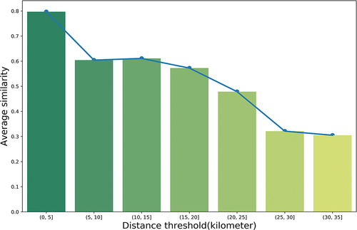
Figure 7. An example of embedding vectors in a road network graph: (a) road networks; (b) embedding vectors of road nodes; (c) spatial distribution of cosine similarities.

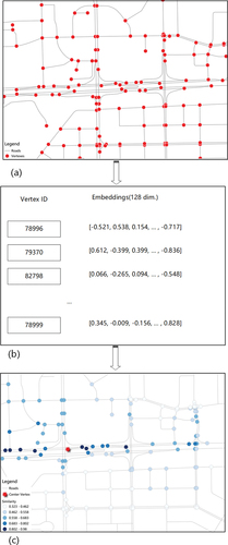
Figure 8. The spatial distribution of hierarchical communities. Note that the solid black lines indicate the administrative boundaries. (a) top-level communities; (b) second-level communities; (c) third-level communities; (d) and (e) indicate the second-level divisions and third-level divisions of Jianghan district.

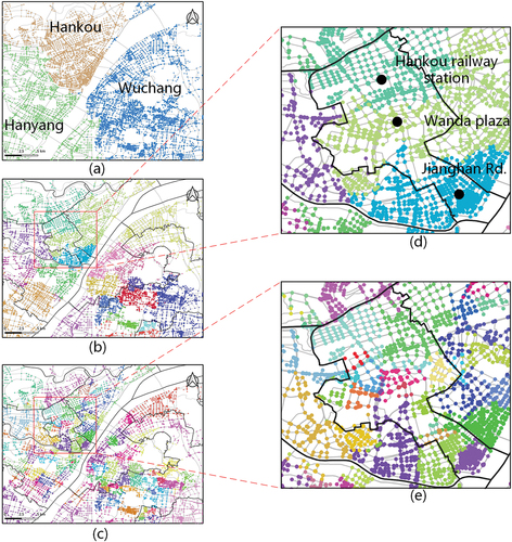
Table 1. Comparison of different communities.

Different communities	Top-level	Second-level	Third-level
Total number of communities	3	22	127
Average edge weight (relatedness)	0.857	0.859	0.864

Figure 9. The chord diagram of traffic flows using origins and destinations of taxi movements. noting that the numbers in the left diagram and right map is consistent and indicate the identifier of the sub-regions. (a) the chord diagram; (b) the spatial distribution of sub-regions. the blue lines indicate the sub-regions boundary generated by Thiessen polygon algorithm.

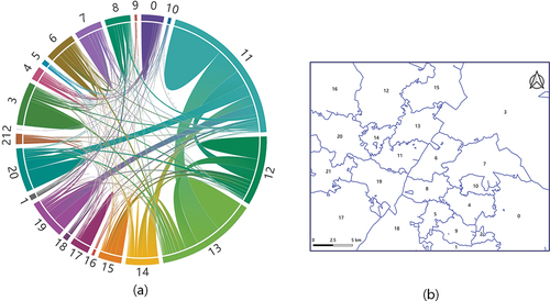
Figure 10. The spatial distribution of urban functional areas based on third-level division.

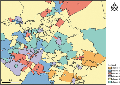
Table 2. Urban functions areas and example locations.

Sub-regional cluster	Function types	Example locations
Cluster 1	Educational area	Huazhong University of Science and Technology
Cluster 2	Comprehensive market area	Qingling Road Materials Market, Wuhan Furniture Store
Cluster 3	Industrial area	Hongqiao Industrial Park
Cluster 4	Business, commercial area	Wuhan International Expo Center
Cluster 5	Residential, commercial area	Donghu Ecological Tourism and Scenic Area, Gangdu Residential Area
Cluster 6	Transportation, business and industrial area	Wuchang Railway Station, Acer Bus Transport Station

Table 3. The percentage of average frequency of taxi flows between the second-level divisions within the same division of seven days.

Methods	9 May 2015	10 May 2015	11 May 2015	12 May 2015	13 May 2015	14 May 2015	15 May 2015
O-Infomap	0.294	0.288	0.312	0.292	0.299	0.297	0.300
D-Infomap	0.339	0.369	0.351	0.374	0.359	0.382	0.366
Proposed method	0.379	0.372	0.391	0.378	0.378	0.384	0.386

Table 4. Indices for mixed land use of the third-level divisions.

Methods	Number of divisions	$R_i$		$H_i$		$D_i$
		Mean	Std.	Mean	Std.	Mean	Std.
O-Infomap	124	105.236	368.350	8.859	35.313	0.945	0.087
D-Infomap	147	55.508	102.843	4.014	6.694	0.953	0.036
Proposed method	127	37.417	64.454	3.156	5.614	0.956	0.037

Data availability statement

The data and codes that support the findings of this study are available from the corresponding author upon reasonable request.