Spatial heterogeneity in the urban household living conditions: A-GIS-based spatial analysis

Figures & data

Figure 1. Location map of the study area. The map showing the selected 146 urban centres, districts boundary and relief.

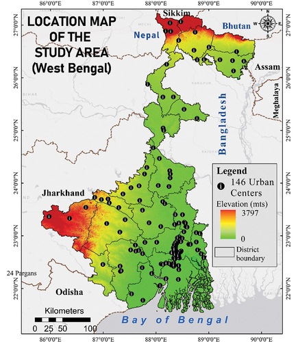
Figure 2. Methodological flowchart adopted for the present study.

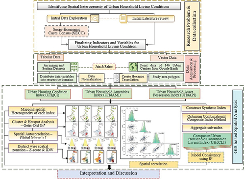
Table 1. Selected dimensions, indicators, and variables for the assessment of Urban Household Condition of Living.

Index	Indicators	Variables Description	Symbol	Relation
Housing Quality Index	House Material	Household Having Houses With Predominant Material Of Wall In Durable Nature	Wall	+
		Household Having Houses With Predominant Material Of Roof In Durable Nature	Roof	+
	Ownership	Household Having Own House	Ownership	+
	Dwelling Room Status	Household Having No Dwelling Room	No Room	-
		Household Having One Dwelling Room	One Room	-
		Household Having More Than One Dwelling Room	More Room	+
Household Amenities Index	Drinking Water	Household Having Availability Of Drinking Water Sources Within The Premises	Drinking Water	+
	Kitchen	Household Having Exclusive Kitchen Availability	Kitchen	+
	Lighting Source	Household Having No Sources Of Lighting	No Light	-
		Household Having Electricity As Main Sources Of Lighting	Electricity	+
	Sanitation	Household Having No Waste Water-Outlet Connections	No Waste Outlet	-
		Household Having Water-Seal Latrine Exclusively For The Household Members	Latrine	+
Household Assets Possession Index	Basic and essential assets	Households Having Refrigerator Availability	Refrigerator	+
		Household Having No Modern Communication Facilities	No Communication	-
		Household Having Computer/Laptop Availability	Computer	+
		Household Having No Motorize Wheelers Availability	No Wheelers	-
		Household Having Air Conditioner (AC) Availability	Air Conditioner	+
		Household Having Washing Machine Availability	Washing Machine	+

Figure 3. Box and whisker plot showing the data characteristics of the selected variables.

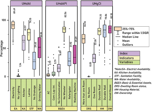
Table 2. Summary statistics of the selected variables.

Variables	Mean	SD	CV	Maximum	Minimum	95% CI Mean
Wall	78.86	16.0	20.23	100	21.1	(76.3,81.4)
Roof	79.25	11.5	14.48	100	38.5	(77.4,81.1)
Ownership	82.10	13.7	16.64	100	0.00	(79.9, 84.3)
No Room	0.05	0.14	299.36	1.42	0.00	(0.0249, 0.0717)
One Room	33.3	11.0	33.08	67.7	4.87	(31.5, 35.1)
More Room	66.6	11.0	16.55	95.1	31.4	(64.8, 68.3)
Drinking Water	51.2	22.0	43.7	100	1.98	(47.6, 54.8)
Kitchen	61.6	16.6	26.89	97.8	24.2	(58.9, 64.3)
No Light	1.34	1.74	130.22	13.3	0.00	(1.05, 1.62)
Electricity	89.69	9.52	10.61	100	57.6	(88.1, 91.2)
No Waste Outlet	29.7	19.9	66.97	95.2	0.00	(26.4, 32.9)
Latrine	74.1	14.4	19.38	100	30.9	(71.8, 76.5)
Refrigerator	31.9	15.7	49.15	85.1	5.04	(29.4, 34.4)
No Communication	16.9	10.8	64.01	52.8	0.72	(15.1, 18.6)
Computer	5.78	5.38	93.91	0.00	37.7	(4.91, 6.66)
No Wheelers	82.6	8.44	10.22	98.6	51.8	(81.2, 83.9)
Air Conditioner	3.79	4.88	128.94	34.5	0.00	(3.00, 4.58)
Washing Machine	39.29	20.5	52.17	97.3	5.77	(36.0, 42.6)

Figure 4. Spatial pattern of selected variables used for the present study. (a-f) Urban housing condition variables which includes predominant material of roof (RF), predominant wall materials (WA), ownership status (OS), No room (NR), one room (OR), and more than one room (MOR); (g-l) Urban household amenities variables which includes drinking water (W), kitchen availability (KT), electricity availability (EL), no electricity (NE), no waste water-outlet (NWO) connections and water-seal latrine facility (LT); (m-r) Urban household asset possession variables which includes availability of air conditioner, refrigerator (RF), no communications (NCM), no motorize wheelers (NW), washing machine (WM) and computer/laptop availability (CL).

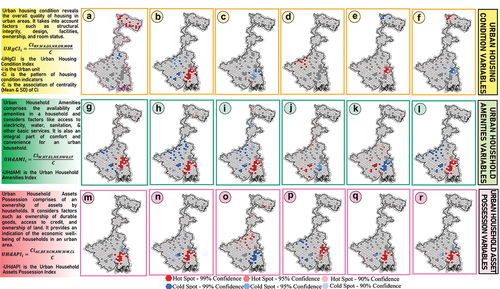
Table 3. Variable-based Moran’s I index, z-score, and pattern of spatial association.

Index	Variable	Moran’s I	z-score	Pattern
Housing Quality Index	Wall	0.29*	21.88	Clustered
	Roof	0.03*	2.96	Clustered
	Ownership	0.02*	1.98	Clustered
	No Room	0.00	0.266	Random
	One Room	0.03*	3.30	Clustered
	More Room	0.03*	3.23	Clustered
Household Amenities Index	Drinking Water	0.15*	11.85	Clustered
	Kitchen	0.22*	17.27	Clustered
	No Light	0.05*	4.72	Clustered
	Electricity	0.33*	25.17	Clustered
	No Waste Outlet	0.17*	12.96	Clustered
	Latrine	0.25*	19.00	Clustered
Household Assets Possession Index	Refrigerator	0.25*	18.78	Clustered
	No Communication	0.31*	23.64	Clustered
	Computer	0.16*	12.90	Clustered
	No Wheelers	0.07*	5.87	Clustered
	Air Conditioner	0.15*	11.75	Clustered
	Washing Machine	0.14*	10.83	Clustered

Note *: the corresponding significance level (p-value) is < 0.001.

Figure 5. Thematic variations of computed sub-indexes (a) Urban Housing Condition index (UHgCI); (b) urban household amenities (UHdAMI); and (c) urban household assets possession (UHdAPI).

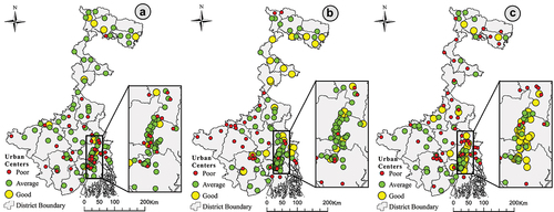
Figure 6. Hotspots & coldspots showing spatial clustering pattern, autocorrelation and zonal distribution of computed sub-indexes. (a-c) UHgCI, (d-f) UHdAMI, (g-i) UHdAPI.

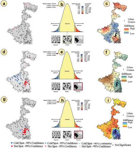
Figure 7. Spatial variation of Composite Urban household condition of living index (UHdCLI). (a) Thematic variation of UHdCLI based on index value, (b & c) spatial pattern and autocorrelation of UHdCLI (d) district wise spatial zonation of UHdCLI.

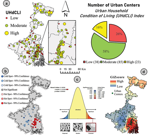
Table 4. Spatial zonation based on GiZ by inverse distance weighted (IDW) interpolation based on urban household condition of living index (UHdCLI).

Spatial Zonation based on GiZ by inverse distance weighted (IDW) interpolation
Zone of High-High Value	Zone of Low-Low Value
(a) Kolkata Municipal Corporation and surrounding urban areas. (b) Majority part of North 24 Paragana, Howrah, Southern Part of Nadia. (c) All most all part of South 24 Paragana, and very small north eastern part of Paschim Medinipur District. (d) Whole Darjeeling, Jalpaiguri, Alipurduar, Coochbehar, and upper most part of Uttar Dinajpur. (51.29%)	(a) Almost all part of Murshidabad, Birbhum, Bankura, Puruliya and Bardhaman district (b) Sparsely identified in Purba and Paschim Medinipur District. (c) Upper part of Nadia, part of Maldah, and Dakshin Dinajpur. (47.56%)

Figure 8. Scatter matrix plot showing the Pearson’s correlation with adjusted R² for the constructed UHgCI, UHdAMI, UHdAPI and UHdCLI. The ellipse showing the distribution of Urban centres with 95% confidence.

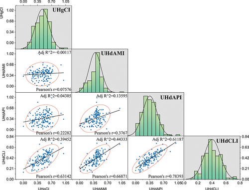
Table 5. Summary of regression analysis for model consistency.

Model	Predictors	Coefficients	R^2	t	Significance
UHdCLI	Roof	.302	0.815	5.330	.000
	No Room	−.169		−2.208	.004
	Electricity	.609		9.308	.000
	No Light	−.293		−4.504	.000
	Air Conditioner	.304		5.358	.000
	Washing Machine	.123		2.139	.034

Data availability statement

The governmental data used in this study is freely available from SECC, India.