Green Cartography: A research agenda towards sustainable development

Figures & data

Figure 1. Estimation of the energy consumption of a Google map with a satellite background (a) and that of a light mode street map (b) on a 2,340 × 1,080 pixel OLED screen.

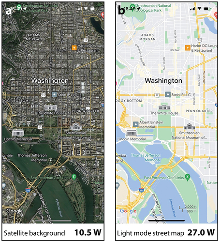
Figure 2. A conceptual framework for green cartography consisting of four dimensions: content, form, use context, and carbon footprint.

Figure 3. A comparison of the energy consumption of four map generalization operators: (a) selection; (b) simplification; (c) smoothing; and (d) aggregation.

Figure 4. A comparison of the energy consumption of four common classification methods. From left to right: equal intervals, quantiles, standard deviations, and natural breaks.

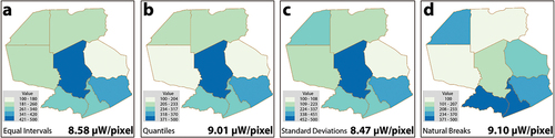
Figure 5. A comparison of the energy consumption of four common interpolation methods: (a) IDW; (b) kriging; (c) natural neighbour; and (d) spline.

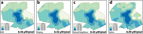
Figure 6. A comparison of the energy consumption of nine map projections on a simple test map with an assumed viewport (all maps are at the same cartographic scale of 1:470,000,000 and have a resolution of 1,770 × 1,600 pixels): (a) stereographic, conformal projection; (b) mercator, conformal projection; (c) hotine, conformal projection; (d) aitoff, arbitrary projection; (e) patterson, arbitrary projection; (f) robinson, arbitrary projection; (g) goode, equal-area projection; (h) behrmann, equal-area projection; and (i) sinusoidal, equal-area projection.

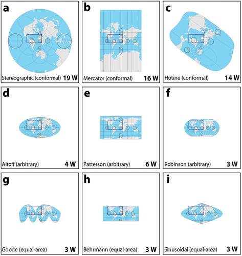
Figure 7. Energy consumption of nine-class colour schemes from colorbrewer.Org: (a) sequential; (b) diverging; and (c) qualitative.

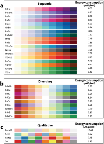
Figure 8. Estimation of the energy consumption of colours over the HSV colour space: (a) all colours; and (b) colour value and saturation transitions for sequential and diverging schemes.

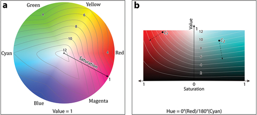
Figure 9. A comparison of the energy consumption of the three symbols at different iconicities: (a) geometric; (b) associative; (c) pictorial.

Figure 10. An estimation of energy consumption on typography with different typefaces, font sizes, and weights exhibiting low and high label densities.

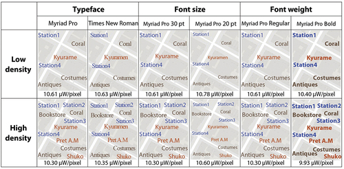
Figure 11. A comparison of the energy consumption of four types of symbolization: (a) dot density mapping; (b) proportional symbol mapping; (c) isarithmic mapping; and (d) choropleth mapping.

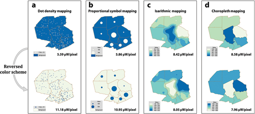
Figure 12. A comparison of the energy consumption of dark mode and light mode with the same map data and same screen setting in terms of brightness and contrast: (a) light mode; (b) dark mode.

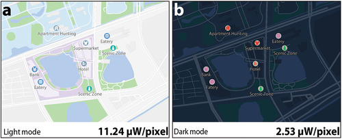
Figure 13. A comparison of the energy consumption of maps with different interfaces: searching interface (a) and (c); navigation interface (b) and (d).

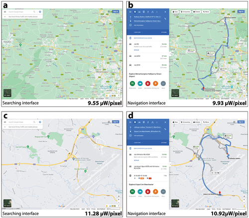
Table 1. Summary of big questions and subquestions on how digital maps can be greener.

Reorganize the map content to save energy
1	How can maps be generalized to save energy?
	A	How can map generalization operators be applied to reduce energy with consideration of both mapping data and map design decisions?
	B	What is the optimal trade-off between the extra energy cost of applying energy-aware generalization techniques against the actual intended reduction of energy consumption?
2	How can the geography of map access be used to reduce energy consumption?
	A	How can geographic patterns of map use be leveraged to render only tiles of interest?
	B	How can specific map locations or regions be prioritized for map tiling under time, bandwidth, and other energy constraints?
3	How can the similarity among map content be used to save energy
	A	How can similarity be used to remove data redundancies among tiles to minimize storage needs?
	B	How can similarity across scales be used for progressive transition between zoom levels?
Adjust the map form to save energy
4	How can the visual and dynamic variable syntactics be extended to save energy?
	A	Can the energy consumption of each visual and dynamic variable be predictably calculated across map use contexts?
	B	How should the visual and dynamic variables be recoupled to the data level of measurement or other design considerations to save energy?
	C	How can iconic reduce their carbon footprint while retaining unique cultural meanings and pluralistic design practices?
	D	How can established colour schemes and symbol sets be modified to save energy?
5	How can thematic maps be redesigned to save energy?
	A	How do data characteristics such as distribution, density, dimensionality, etc., impact the energy consumed by thematic maps?
	B	How should recommendations for selecting and designing different thematic map types be revised to save energy?
6	How can a map interfaces and interactions be redesign to save energy?
	A	How can the interface style, scope, and freedom adapt to reduce energy consumption?
	B	How can the energy consumption of interaction operators be estimated?
	C	What is the optimal compromise beween energy-aware map interfaces and the utility, usability, and satisfaction of the user experience?
Refine the map-use context to save energy
7	How can the carbon footprint be reduced in different map-use contexts?
	A	How can the carbon footprint be minimized while maximizing and preserving functionality for general map-use contexts?
	B	What considerations for energy-aware map content and form can be exposed to users as customizable settings?
8	How does energy-aware design impact digital map reading?
	A	How do green maps influence the reader’s affective and aesthetic response?
	B	How do green maps impact our perception and the quality of map communication?
9	How can the attitude towards using energy-aware maps be developed?
	A	How can individual, organizational, and social attitudes be shaped to bridge the gap between designing and using greener maps?
	B	How can emotions towards, behaviours with, and reasoning about energy-aware maps be improved to enable uptake of greener maps?

Data availability statement

Data available upon request from the authors.