Flood map boundary sensitivity due to combined effects of DEM resolution and roughness in relation to model performance

Figures & data

Figure 1. Location of test sites in black: (a) the Voxna river in Edsbyn and (b) the Testebo river north of the city of Gävle. ©Lantmäteriet.

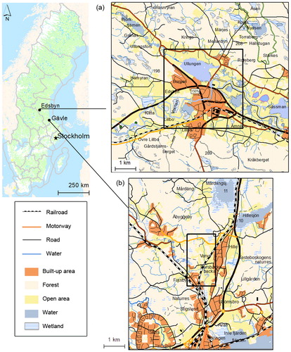
Figure 2. The different DEMs used for the simulations: (a) the Testebo river and (b) the Voxna river. Direction of flows is shown by the arrows.

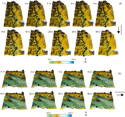
Figure 3. Illustration of how the points used for disparity measurements were sampled from one of the simulation results (left) and from the reference data (right) using the cross-sections.

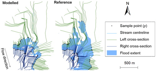
Figure 4. Flood extents grouped according to DEM resolution for the Testebo river.

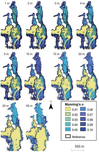
Figure 5. Flood extents grouped according to DEM resolution for the Voxna river.

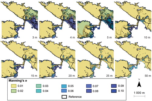
Figure 6. The water levels produced from using different resolution DEMs and Manning’s $n$ for two coss-sections characterized by steep (CS #10) and flat (CS #42) side slopes in the Testebo river.

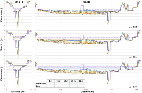
Figure 7. Cross-sectional profiles of the Voxna river. CS #32 is from a location bounded by steep-side slope, while CS#14 was from a flatter part of the river.

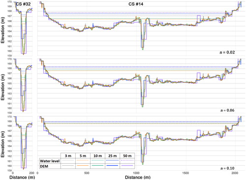
Figure 8. Performance contours for the feature agreement statistics ($F1$ and $F2$) and the two disparity measures (mean disparity, $\overline{D};$ and median disparity, $\stackrel{\sim }{D}$) for simulation results from (a) Testebo and (b) Voxna rivers. High model performances are represented by lighter brown colour, while low performances are darker.

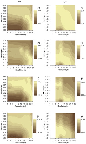
Figure 9. Size differences between the simulated (blue) and the actual (black outline) floods for (a) the Testebo river and (b) the Voxna river. Underestimation of the actual flooding is occurring when the black circle is larger than the blue one, while overestimation is occurring when the blue is larger than the black outline.

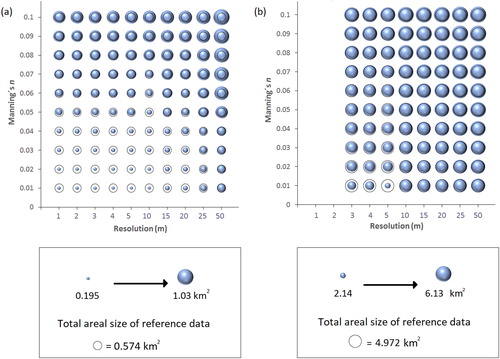
Figure 10. Variations in extents produced for the least (top) and most (bottom) optimal performances for Testebo river (a) and Voxna river (b).

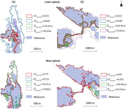
Figure 11. Flood extents for the highest performing DEM resolution and Manning’s $n$ combinations for the Testebo river.

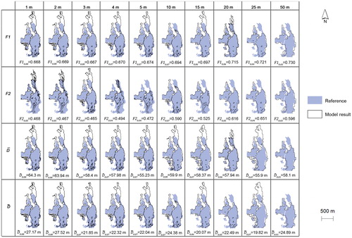
Figure 12. Flood extents for the highest performing DEM resolution and Manning’s $n$ combinations for the Voxna river.

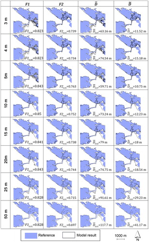
Figure 13. Interval plots for the DEM and Manning’s $n$ for the Testebo (a) and Voxna (b) rivers. The mean performance for each resolution/Manning’s $n$ is marked as blue square.

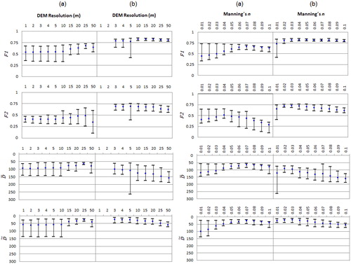
Figure 14. Histogram of performance measures for the 100 simulation results of the Testebo river (a), and the 80 simulation results of the Voxna river (b). The dashed line represents using the threshold of $F\ge$0.50 and $D\le$50 m.

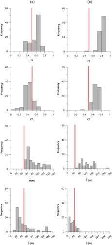
Table 1. Comparison of best performance results among different variants of feature agreement statistics, for the Testebo and Voxna rivers.

	Testebo				Voxna
Res. (m)	$F1$	$F2$	${F2}_U$	$F3$	$F1$	$F2$	${F2}_U$	$F3$
1	0.668[n=0.08]	0.468[n=0.05]	0.607[n=0.10]	0.337[n=0.08]	–	–	–	–
2	0.669[n=0.08]	0.467[n=0.05]	0.601[n=0.09]	0.339[n=0.08]	–	–	–	–
3	0.667[n=0.08]	0.465[n=0.07]	0.604[n=0.09]	0.333[n=0.08]	0.823[n=0.08]	0.739[n=0.03]	0.787[n=0.09]	0.646[n=0.08]
4	0.670[n=0.07]	0.494[n=0.04]	0.608[n=0.09]	0.340[n=0.07]	0.823[n=0.08]	0.734[n=0.04]	0.787[n=0.09]	0.647[n=0.08]
5	0.674[n=0.07]	0.472[n=0.04]	0.605[n=0.09]	0.348[n=0.07]	0.843[n=0.08]	0.763[n=0.05]	0.802[n=0.08]	0.687[n=0.08]
10	0.694[n=0.07]	0.590[n=0.07]	0.622[n=0.08]	0.388[n=0.07]	0.85[n=0.04]	0.752[n=0.03]	0.807[n=0.04]	0.700[n=0.04]
15	0.697[n=0.06]	0.525[n=0.04]	0.638[n=0.08]	0.395[n=0.06]	0.841[n=0.04]	0.738[n=0.02]	0.805[n=0.06]	0.682[n=0.04]
20	0.715[n=0.06]	0.616[n=0.05]	0.630[n=0.08]	0.430[n=0.06]	0.843[n=0.03]	0.744[n=0.02]	0.803[n=0.04]	0.686[n=0.03]
25	0.721[n=0.04]	0.651[n=0.04]	0.645[n=0.07]	0.446[n=0.04]	0.828[n=0.02]	0.715[n=0.01]	0.790[n=0.03]	0.655[n=0.02]
50	0.730[n=0.03]	0.596[n=0.03]	0.646[n=0.01]	0.460[n=0.03]	0.828[n=0.01]	0.697[n=0.01]	0.793[n=0.03]	0.657[n=0.01]