
Figures & data
Figure 1. Location of the study area in China (left: Google Maps), the Xulong gully (right).
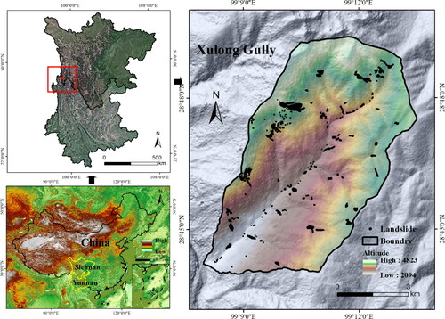
Figure 2. Architecture of the datasets, their derived products, and their usage.
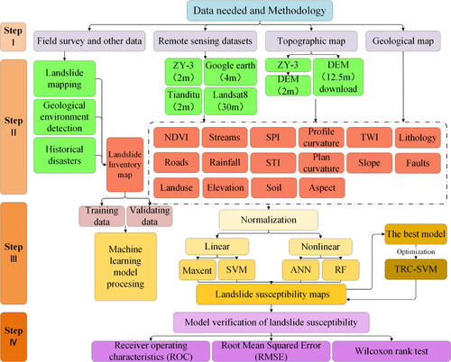
Figure 3. Examples of collapses and landslides: (a)-(c) landslide from an optical image (d) - (f) are landslides from field investigation.
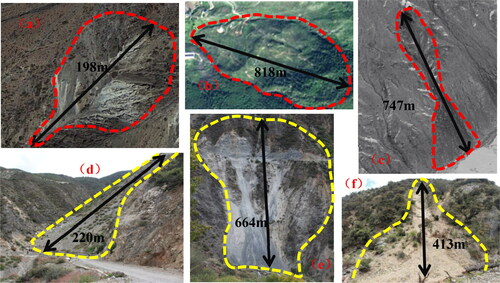
Figure 4. Landslide casual factors: (a) Aspect; (b) Plan curvature; (c) Profile curvature; (d) Slope; (e) Elevation; (f) Distence to streams; (g) NDVI; (h) Distance to faults; (i) Distance to roads; (j) TWI; (k) Lithology; (l) Landuse; (m) SPI; (n) STI; (o) Precipitation; (p) Soil.
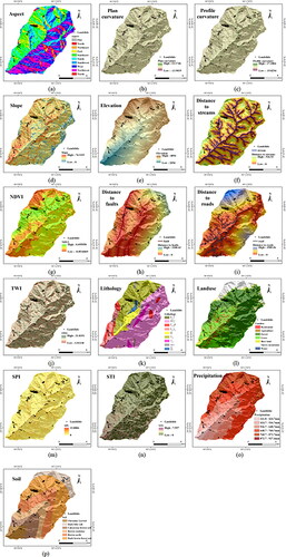
Figure 5. The diagram of SVM classification principle: (a) Map of linear classification; (b) Sketch map about linear classification of SVM.
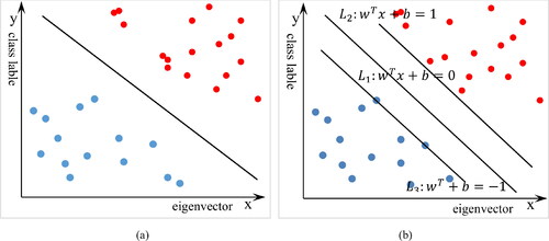
Figure 6. The architecture of ANN.
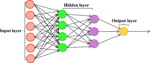
Figure 7. The principle chart of RF.
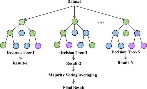
Figure 8. The relevance of landslide factor (DTF is distance to faults, DTR is distance to roads, DTS is distance to streams Pla is Plan Curvature, and Pro is profile curvature).
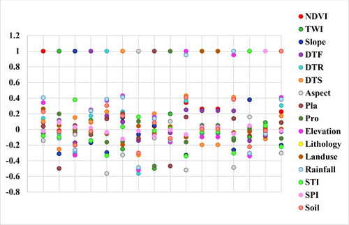
Figure 9. The weight of every landslide sensitivity factor in Maxent, SVM, ANN and RF models.
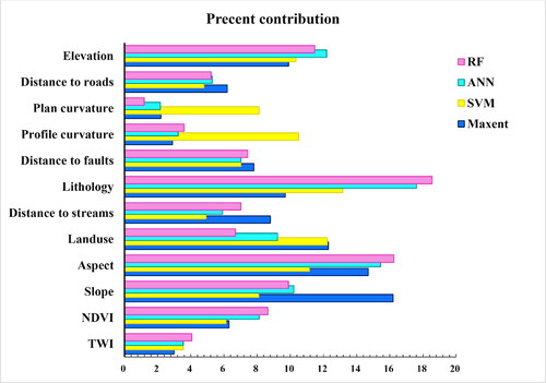
Figure 10. Landslide susceptibility maps using (a) Maxent; (b) SVM; (c) ANN; (d) RF.
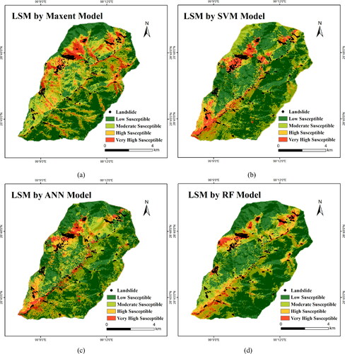
Table 1. Classification results and landslide pixels leading to corresponding FR values of the four models.
Table 2. Comparison of the four models.
Figure 11. ROC curves and AUC values using training dataset and validation dataset:(a)training dataset; (b) validation dataset.
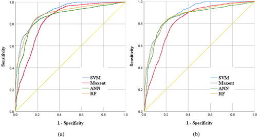
Figure 12. Landslide susceptibility map using TRC-SVM.
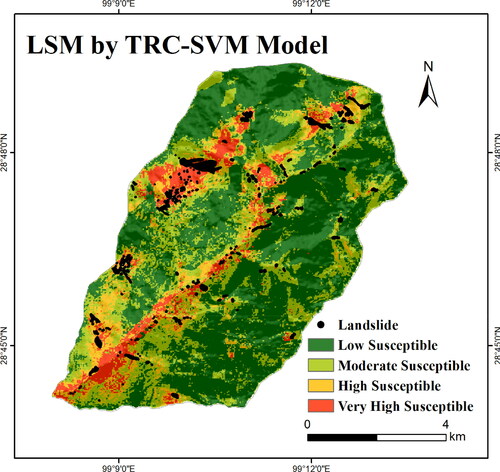
Figure 13. ROC curves and AUC values using training dataset and validation dataset:(a)training dataset; (b) validation dataset.
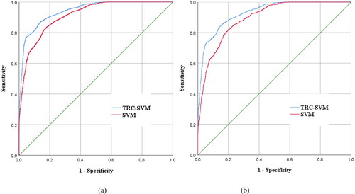
Table 3. Comparison of the SVM and TRC-SVM.
Figure 14. Detailed classification in VH of the top five conditioning factors for the four models.
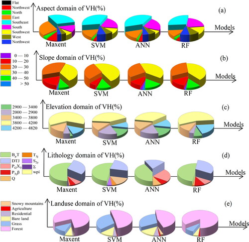
Table 4. Spatial relationship between landslides, conditional factors, and LSM.
Data availability statement
Not applicable.