Reconstruction of liquefaction damage scenario in Northern Bihar during 1934 and 1988 earthquake using geospatial methods

Figures & data

Figure 1. The major thrust faults, lineaments, and faults overlayed on the study area and the Satellite (Landsat OLI) image depicting the Northern Bihar region used for the liquefaction hazard assessment.

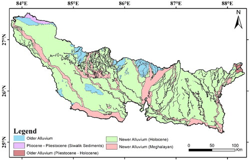
Figure 2. The lithological map of the study area showing different geological units classified in older alluvium from Pliocene to newer alluvium Meghalayan (BHUKOSH, GSI).

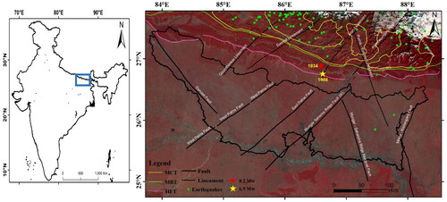
Figure 3. Modified Mercallie Intensity map shown for 1934 earthquake (a) Modified after Kayal. (2010), and 1988 earthquake (b) Modified after GSI., 1993, Prajapati et al. (2017).

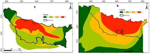
Table 1. Thematic layers and their importance in preparing the liquefaction susceptibility map.

Thematic layer	Liquefaction susceptibility	Data source
Groundwater table	The average water table depth for soil liquefaction is 2.05 m (Hartantyo, 2006), the water table depth was classified for the degree of hazard using the classification provided in (Chung & Rogers, 2013). Soil saturated with groundwater is susceptible to liquefaction (Bozzoni et al. 2021). The range of groundwater depth was adopted is 0–1.4 (Very highly susceptible), 1.4–3.2 (moderately susceptible), 3.2 − 4.5 (moderately susceptible), 4.5 − 7.4 (low susceptibility), >7.4 (none)	Central Ground Water Board online Portal
Structure density	The structures control the circulation and storage of groundwater, and these constitute secondary porosity (Pudi et al. 2019; Takorabt et al., 2018). A site near the structures receives more energy relative to a distant location. Classification of structure density for liquefaction susceptibility map was done using natural break application of ArcGIS. The range was distributed such as 13 (low susceptibility) > 23 (moderate susceptibility) > 38 (moderate susceptibility)> 62 (highly susceptible)> 119 (very highly susceptible)	BHUKOSH (GSI)
Soil texture	Sandy and loamy soils have relatively better water infiltration rates 20-30 mm/hr than clay-rich soils 1-10 mm/hr https://www.fao.org/3/s8684e/ s8684e0a.htm. Soil texture classification suggested in (https://www. geospatialworld.net/article/the-study-for-assessment-of-susceptibility-to-soil- liquefaction-in-taiwan/) was used in this study. The soil texture divided into coarse texture (Very highly susceptible ), medium coarse texture (highly susceptible), medium texture (moderate susceptibility), medium fine texture (moderate susceptibility), fine clay silt (Low susceptibility)	NBSS, Nagpur
Drainage buffer	Liquefaction is generally observed along the drainage (Zhu et al. 2015, 2017; Pudi et al. 2019; Bozzoni et al. 2021). The drainage buffer classified as 0–500 m from the drainage liquefaction likely, 500–1000 m liquefaction possible, and >1000 liquefaction not likely	SRTM DEM, 30m USGS
Age of deposits	Liquefaction susceptibility decreases as the alluvial and flood plains’ geologic age increases (Dobry, 1985). Meghalayan deposits are the recent deposits less than age < 10,000 yrs hence least compacted and susceptible to liquefaction. In this study, the age of deposits classified as Pliocene-Pleistocene (very low susceptibility), pleistocene (low susceptibility), Holocene (moderate susceptibility) and Meghalayan (highly susceptible). Recent deposits are common along rivers, so the drainage buffer is essential for liquefaction estimation.	BHUKOSH (GSI)
Geomorphology	Geomorphological units in the study area classified as dissected hills & valleys (very low susceptibility), piedmont slope (low susceptibility), older alluvial plain (moderate susceptibility), younger alluvial plain (highly susceptible) and active flood plain (very high susceptible)	BHUKOSH (GSI)

Table 2. Pairwise comparison matrix for site-specific parameters used to prepare the liquefaction susceptibility map.

	Groundwater	Structure density	Soil texture	Drainage buffer	Age of deposits	Geomorphology	Eigen Vector
Groundwater	1	2	3	4	4	5	0.35
Structure density	0.5	1	3	4	5	5	0.28
Soil texture	0.33	0.33	1	2	3	5	0.15
Drainage buffer	0.2	0.25	0.5	1	2	3	0.09
Age of deposits	0.25	0.2	0.33	0.5	1	2	0.06
Geomorphology	0.2	0.2	0.25	0.33	0.5	1	0.04
Total	2.48	3.98	8.08	11.83	15.5	21

Note: This analysis estimates the highest weightage 0.34 for groundwater and the lowest weightage 0.04 for geomorphology.

Figure 4. Input layers used for liquefaction susceptibility evaluation using rapid response and loss estimation model (Zhu et al. 2017), (a) precipitation, (b) groundwater, (c) distance to water body, (d) shear wave, (e) PGV 1934, and (f) PGV 1988.

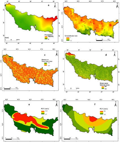
Figure 5. Input thematic layers used in the AHP model are (a) structure density, (b) soil texture, (c) geomorphology, (d) drainage buffer, (e) groundwater and (f) age of deposits. The GIS layers were scaled according to the degree of the liquefaction.

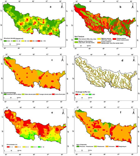
Figure 6. The PGA map prepared from the isoseismal map a) 1934 earthquake event 8.2 Mw (Kayal 2010) and (b) 1988, 6.9 Mw (Mukarjee and Lavania 1998). The PGA is in cm/sec². It is observed from the map that for 1934 high PGA values were observed than the 1988 event.

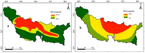
Figure 7. (a, b) shows the liquefaction damage scenario during the 1934 earthquake using Model A and Model B, and (c, d) shows the liquefaction scenario during 1988 by model A and model B, respectively. The maps were classified into four zones such as very low, low, high and severe using a natural break in ArcGIS 10.5.

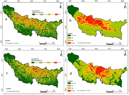
Table 3. RMSE determined for separate classes (very low, low, high and severe) in the liquefaction hazard map from the reference location.

	RMSE
Classes	1934 Model A	1934 Model B	1988 Model A	1988 Model B
Very low	1.21	0.38	0.76	0.26
Low	0.32	0.15	0.33	0.13
High	0.19	0.05	0.05	0.03
Severe	1.51	0.22	1.22	0.08

Notes: The RMSE describes how close the predicted value with the reference value. The ‘high’ class of the AHP model has the lowest RMSE value than other classes, which infers that the predicted liquefaction high zone is close to the reference liquefaction zone.

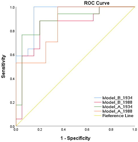
Figure 8. The ROC curve generated using the SPSS tool shown for 1934 and 1988 earthquake for both models (a, b) the highest AUC found 0.94 for 1934 earthquake using Model B.

Kayal JR. 2010. Himalayan tectonic model and the great earthquakes: an appraisal. Geom Nat Haz Risk. 1(1):51–67.

 Web of Science ®Google Scholar

Prajapati, Sanjay K., Harendra K. Dadhich, Sumer Chopra. 2017. Isoseismal map of the 2015 Nepal earthquake and its relationships with ground-motion parameters, distance and magnitude. J Asian Earth Sci. 133:24–37.

 Web of Science ®Google Scholar

Hartantyo, Eddy, S. K. 2014. Brotopuspito. Correlation of shallow groundwater levels with the liquefaction occurrence cause by May 2006 earthquake in the south volcanic‐clastic sediments Yogyakarta, Indonesia. Int J Appl Sci. 1:1–8.

 Google Scholar

Chung, Jae-Won, J. David Rogers. 2013. Influence of assumed groundwater depth on mapping liquefaction potential. Environ Eng Geosci. 19(4):377–389.

 Web of Science ®Google Scholar

Bozzoni F, Bonì R, Conca D, Lai CG, Zuccolo E, Meisina C. 2021. Megazonation of earthquake-induced soil liquefaction hazard in continental Europe. Bull Earthq Eng. 19(10):4059–4082.

 Web of Science ®Google Scholar

Pudi R, Martha TR, Roy P, Vinod Kumar K, Rama Rao P. 2019. Regional liquefaction susceptibility mapping in the Himalayas using geospatial data and AHP technique. Curr Sci. 116(11):1868–1877.

 Web of Science ®Google Scholar

Takorabt, Mebarka, et al. 2018. Determining the role of lineaments in underground hydrodynamics using Landsat 7 ETM + data, case of the Chott El Gharbi Basin (western Algeria). Arab J Geosci. 11(4):1–19.

 Web of Science ®Google Scholar

Zhu J, Baise LG, Thompson EM. 2017. An updated geospatial liquefaction model for global application. Bull Seismol Soc Am. 107(3):1365–1385.

 Web of Science ®Google Scholar

Dobry, R. 1985. Liquefaction of soils during earthquakes, national research council (nrc), committee on earthquake engineering. Washington (DC): National Academy Press. Report No. CETS-EE-001.

 Google Scholar

Mukarjee S, Lavania BVK. 1998. Soil Liquefaction in Nepal-Bihar Earthquake of August 21, 1988. International Conference on Case Histories in Geotechnical Engineering. 11:587–592. http://scholarsmine.mst.edu/icchge/4icchge/4icchge-session03/11.

 Google Scholar

Data availability statement

The data used to support the findings in this study will be available by the corresponding author upon reasonable request. Restrictions are applied to data, such as Soil Texture which is not freely available.