
Figures & data
Figure 1. Rainfall stations used in the study area.
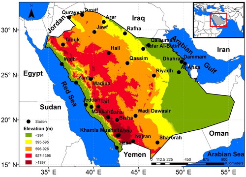
Figure 2. Maximum, mean, and standard deviation of monthly rainfall depth for the stations in the current study with 90%, 95% and 99% percentiles.
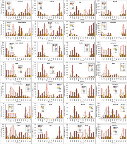
Table 1. Rainfall stations were used in the current study.
Table 2. The common pdfs, f(x), used in the analysis.
Figure 3. Spatiotemporal distribution of the maximum monthly rainfall depth for the stations in the current study from January to December.
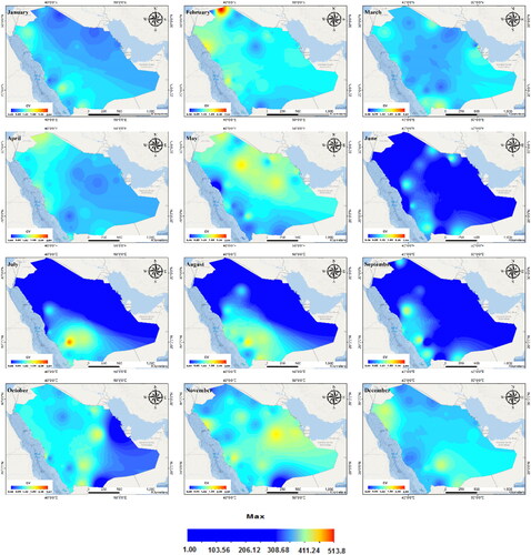
Figure 4. Spatiotemporal distribution of the median of the monthly rainfall depth for the stations in the current study from January to December.
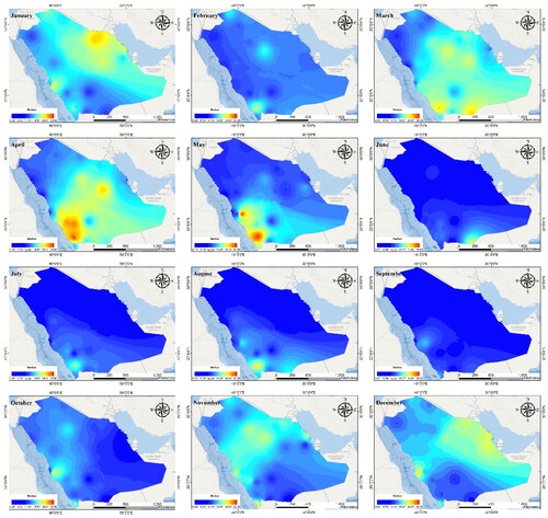
Figure 5. Spatiotemporal distribution of the monthly coefficient of variation (CV) for the stations in the current study from January to December.
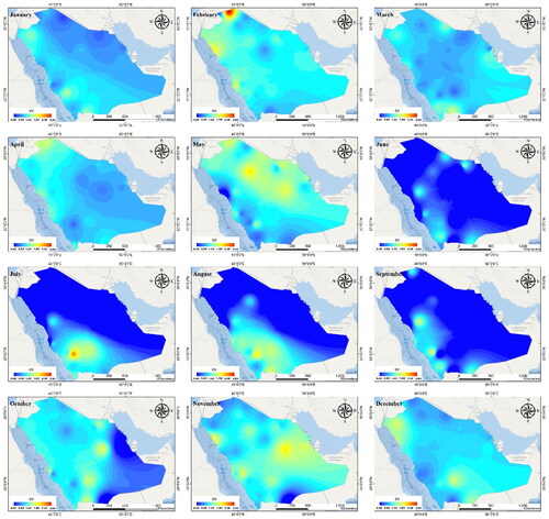
Figure 6. Spatiotemporal distribution of the monthly skewness for the stations in the current study from January to December.
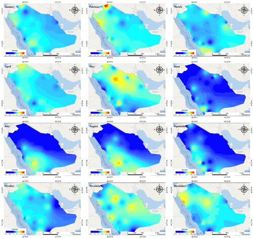
Table 3. Summary statistics.
Figure 7. Comparison between the theoretical CDF and the empirical probability distribution of Taif monthly rainfall.
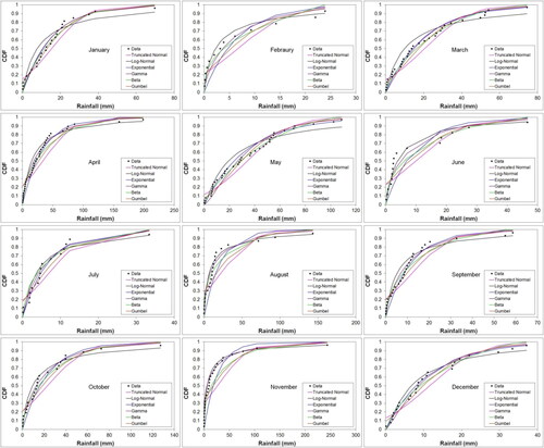
Table 4. Results of the K-S test for the rainfall distributions over the stations and the months of the year.
Figure 8. Sample of the comparison between the theoretical frequency histogram and the frequency histogram of the data for Chi2 test: Abha station from January to December.
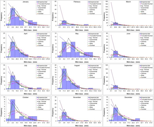
Table 5. Results of the Chi-square test for the rainfall distributions over the stations and the months of the year.
Table 6. Percentage of the fitting distributions based on K-S test of the twelve months for KSA stations.
Table 7. Percentage of the fitting distributions based on Chi2 test of the 12 months for KSA stations.
Table 8. Summary of the test statistics over KSA stations for the 12 months.
Figure 9 . a. L-moment diagram for L-skewness (L-Skew) and L-kurtosis (L-Kurt) ratios: (a) dry season for all stations, (b) wet season over all stations, (c) average over all months, (d) average over all stations. Months that have data less than 3 values with the month at some stations are omitted from the figure. b. Relationship between kurtosis (Kurt) and skewness (Skew) over the months.
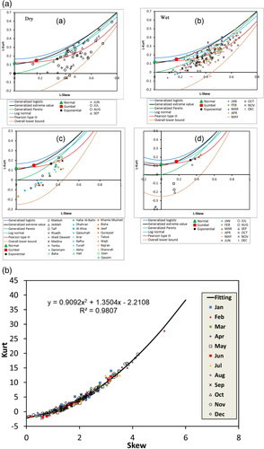
Figure 10. Eigenvalue spectrum (%) of the covariance matrix of rainfall for Dry (upper) and Wet (lower) seasons. The vertical bar shows the uncertainty estimates based on rule of thumb. The leadings 25 eigenvalues are shown.
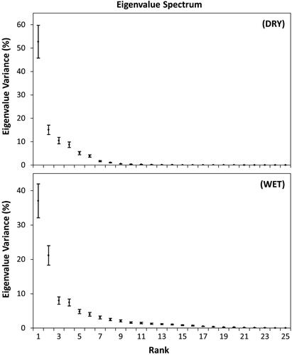
Figure 11. (a) Spatiotemporal distribution of the first leading mode of EOF analysis on the interannual variation of June – September (Dry) rainfall. (b) Same as (a), except for the Wet (November – April) season.
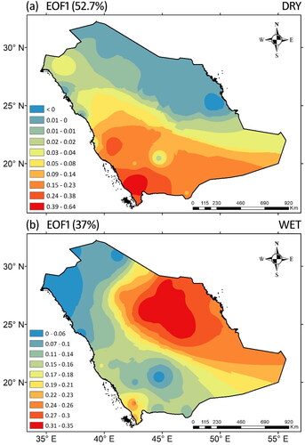
Figure 12. (a & b) Correlation (%) of detrended PC1 of rainfall with SST (HadISST) for Dry (JJAS) and Wet (NDJFMA) seasons, respectively for the period 1985 – 2012. The dotted regions show values at 5% significance level.
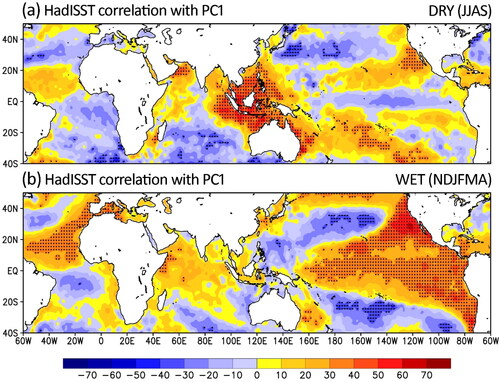
Figure 13. (a) Time series of PC1 of rainfall for dry season over KSA and the average Dipole Mode Index (DMI) during 1985 – 2012. (b) Same as (a), except for the Niño 3, Niño 3.4, and Niño 4 indices for wet season. (c) Same as (b), except for Pacific Decadal Oscillations (PDO) index. All the values of the correlations between PC1 of rainfall and climate indices are statistically significant at 95% level.
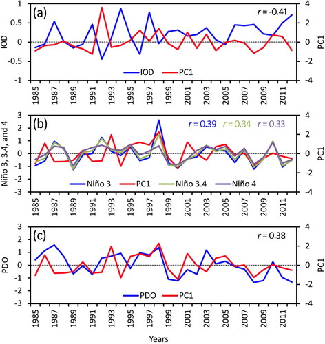
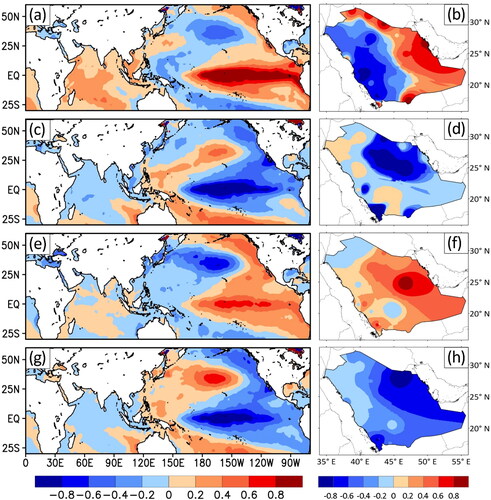
Figure 14. (a and b) El Niño composite of SST and rainfall anomalies, respectively, for wet season. (c – d, e – f, and g – h) Same as first row, except for La Niña, Warm PDO, and Cold PDO composites, respectively. Units are degrees Celsius (°C) for SST and mm/month for rainfall.
Data availability statement
The authors have no permission to submit the data since it belongs to the ministry.