Prediction analysis of landslide displacement trajectory based on the gradient descent method with multisource remote sensing observations

Figures & data

Figure 1. Flow chart of the method for predicting the direction and trajectory of the main slide in a landslide subregion.

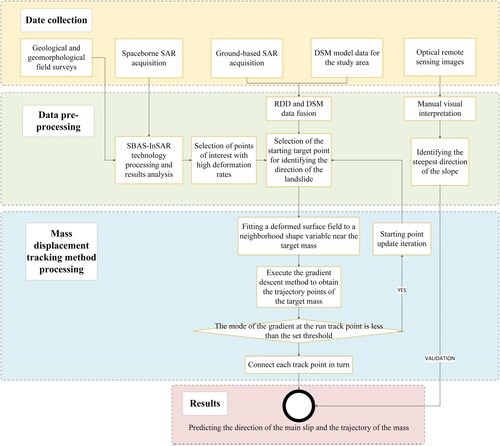
Figure 2. (a) Time–position of Sentinel-1A image interferometric pairs; (b) time–baseline of Sentinel-1A image interferometric pairs. (The yellow point denotes the supermaster image. Blue lines represent interferometric pairs. Green diamonds denote slave images.).

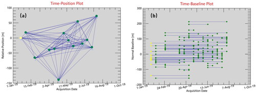
Figure 3. Schematic diagram of RDD and DSM data fusion. (a) 3 D model of the GB-InSAR system observation geometry; (b) GB-InSAR plane geometry model in a range–azimuth coordinate system.

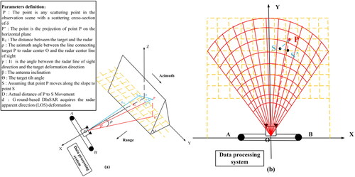
Table 1. Detailed parameters and fitting results of the model.

Surface fitting model	Iterative algorithm	Freedom	Model parameters						R^2
			z0	A	xc	w1	yc	w2
Lorentz2D	Levenberg–Marquardt	1018	−1.723	745.907	103.396	6.431E-5	27.037	5.227E-5	0.86889

Figure 4. Location and shape of the Hongshiyan landslide: (a) Map of the Hongshiyan landslide; (b) presliding and postsliding images for the landslide based on GF-1; (c) after the Ludian earthquake on 5 August 2014; UAVs took aerial photos of the landslide; (d) schematic diagram of area division.

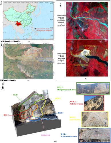
Table 2. The parameters of the M600-Pro-type UAV and Zenmuse-X5 camera lenses.

UAV flight capability	Actual endurance	Aerial camera	Camera parameters
Maximum flight altitude	2500	Effective pixel	16 megapixels
Maximum allowable wind speed	8 m/s	Equivalent focal length	30 mm
Maximum pitch angle	25°	Camera memory	64 GB
Task load	6 kg	Maximum resolution	4608 × 3456

Table 3. Equipment technical index.

Frequency	Bandwidth (MHZ)	Monitoring scope (°)	Operating distance (km)	Repetition time (min)	Range resolution (m)	Azimuth resolution (mrad)
Ku	500	30 ∼ 80	Maximum 5	4 ∼ 10	$\Delta R=\frac{C}{2B}$ = 0.3	${\delta }_{\mathit{angle}}=\frac{\lambda }{2L_s}\gamma$ = 5.4

Figure 5. Monitoring-area radar images (left, middle) and UAV image (right).

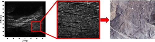
Figure 6. (a) and (b) Deformation rate map (LOS direction) from January 2019 to August 2019; (c) deformation rate map (slope direction) from January 2019 to August 2019; (d) deformation rate map (vertical direction) from January 2019 to August 2019.

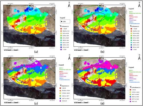
Table 4. SBAS-InSAR versus GPS monitoring data validation (mm/yr).

Point number	Vvertical	Vz	Difference
P1	−19.2784	−12.7841	6.4943
P2	−25.7519	−14.0427	11.7092
P3	−19.6571	−13.1125	6.5446
P4	−65.8456	−46.2145	19.6311
P5	−125.7324	−105.9572	19.7752
P6	−116.7417	−105.4218	11.3199
P7	−103.5482	−91.8849	11.6633
P8	−99.4185	−84.1204	15.2981
P9	−105.7418	−94.5486	11.1932
P10	−127.7716	−114.9813	12.7903

Figure 7. Cumulative displacement map of GB-InSAR campaigns.

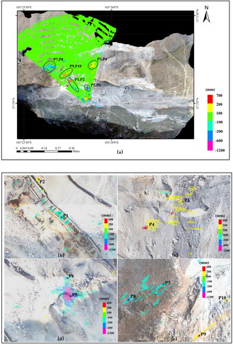
Figure 8. Response of SBAS-InSAR time-series deformation results to rainfall for typical feature points A, B, C, D, and E.

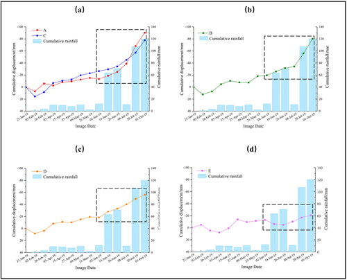
Figure 9. Cumulative deformation curves (a–f) and displacement velocity versus curves (a’–f-) over time at typical monitoring features.

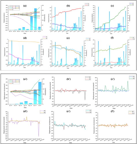
Figure 10. Results of deformation surface field fitting. (a) 3 D scatter plot of the deformation region; (b) schematic of the real deformation region; (c) 3 D smoother fit of the regional deformation field; (d) regional deformation surface field fitted with the Lorentz2D function.

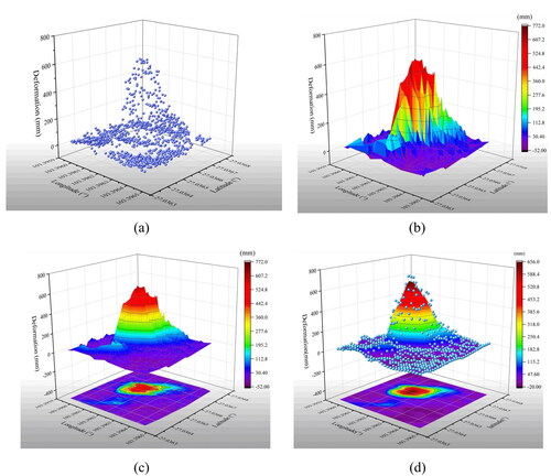
Figure 11. (a) Fitted deformation surface field contours and target starting point maps; (b) predicted main slip direction and displacement trajectory maps.

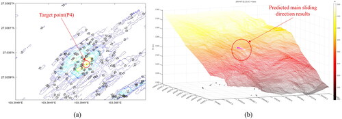
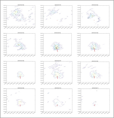
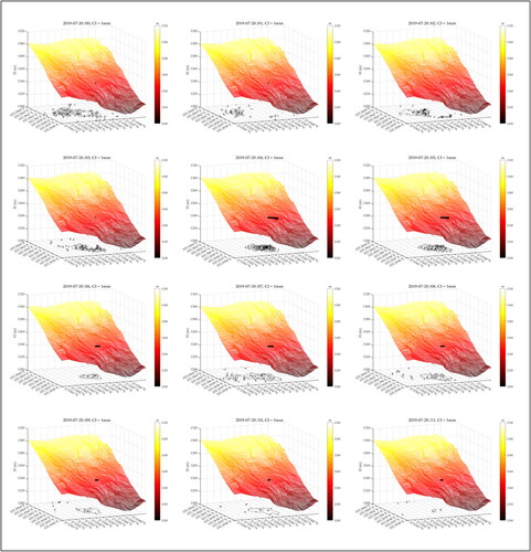
Figure 13. General drawing of displacement tracking and trajectory prediction of 0–12 points on July 20, 2019.

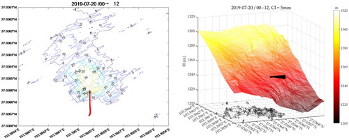
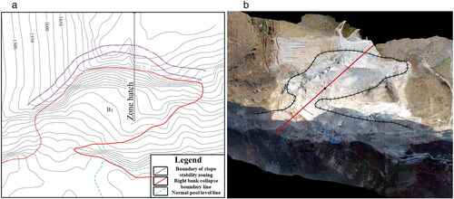
Figure 14. (a) Diagram of the slope stability zone of the right bank collapse; (b) schematic diagram of the main sliding direction of the landslide obtained by the empirical method.

Data availability statement

Self‐collected datasets that support the findings of this study are available from the corresponding author upon reasonable request.