A local regression approach to analyze the orographic effect on the spatial variability of sub-daily rainfall annual maxima

Figures & data

Figure 1. Visual representation of the three approaches used to handle the extrapolation effect described in Section 2.4 for the estimation of the average annual maximum rainfall depth h_d at the elevation z*. The black line represents the fit of the local sample; the vertical grey bars in case (b) and (c) represent the case of extrapolation e_max = 100 m allowed.

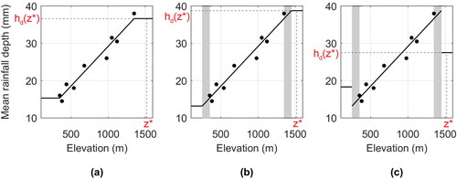
Figure 2. Elevation data (a) and number of rain gauges available for each cell within a 15 km radius (b). Source: Shuttle Radar Topography Mission (Farr et al. 2007).

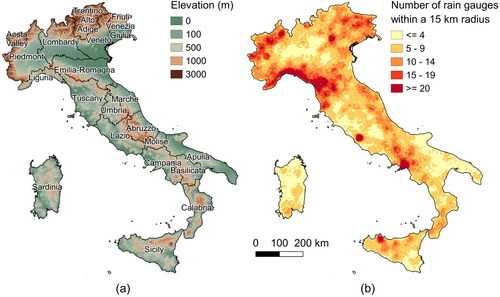
Table 1. Mean, median, modal and standard deviation values of the rain gauges falling in circles of variable radius.

Radius (km)	Mean (n° of stations)	Median (n° of stations)	Mode (n° of stations)	Standard deviation (n° of stations)
10	3.9	3	2	2.7
15	8.2	7	5	5.2
20	14.3	13	7	8.4
25	21.8	19	14	12.2

Figure 3. Average annual maxima of 1 h duration computed on the basis of the 5 nearest stations (a). Residuals of the 1 h model, with an indication of the elevation (b). Box plots of measured and estimated mean of 1 h values (c).

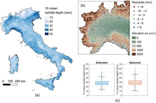
Figure 4. Visual representation through box plots of the slope coefficients obtained with a regression model based on r = 15 to 50 km and Δz = 0 or 100 m in the case of 1 (a) and 24 h durations (b). Please note that Δz is the minimum difference in elevation among the rain gauges of the local sample required to apply the regression.

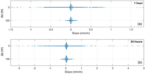
Figure 5. Elevation map with the indication of the area investigated (a). 24 h average annual maxima estimated using radii variable from 15 to 50 km (simulation with an extrapolation of 100 m allowed and with mean rainfall depth evaluated using the 5 nearest rain gauges in uncovered cells) in the case of Δz = 0 m (c) and Δz = 100 m (e) and related slope coefficients (b and d). Red circles in (c) serve to highlight artifacts. Grey color defines areas where the local regression approach is not applicable e.g. due to the impossibility of pooling at least 5 rain gauges or to the lack of significance of the regression model.

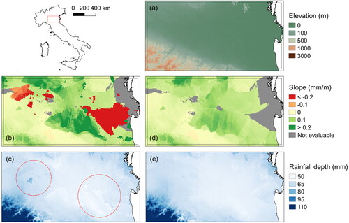
Figure 6. Elevation data for Friuli Venezia Giulia (a) and Sicily (b). In (c, d) extrapolation is allowed without limits and red areas represent cells with negative estimated rainfall. In (e, f) extrapolation is limited to 100 m.

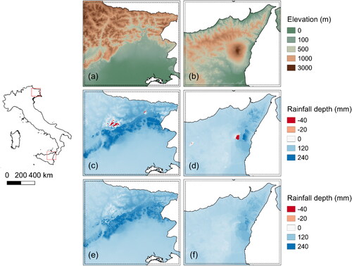
Table 2. Most relevant model configurations.

Case	n (-)	Δz (m)	Radius configuration	rfix (km)	rmin (km)	rmax (km)	emax (m)	Extrapolation configuration (Section 2.4)
0	5	0	Variable	–	–	–	–	–
1	5	100	Variable (V1)	–	1	15	0	a
2	5	100	Variable (V1)	–	1	15	0	c
3	5	100	Variable (V2)	–	15	50	100	c
4	5	100	Fixed	15	–	–	100	b
5	5	100	Fixed	15	–	–	100	c
6	5	100	Fixed	20	–	–	100	c
7	5	100	Fixed	25	–	–	100	c

Case 0 represents the case with mean values reconstructed using the 5 nearest stations, while all the other tests were performed using georegression models. The last column refers to the configuration described in Section 2.4: in configuration ‘a’ extrapolation is not allowed while in ‘b’ and ‘c’ the extrapolation is allowed up to e_max (for the grid cells that would require extrapolation higher than e_max, in configuration ‘b’ the predicted value is set equal to the value obtained by the model at an elevation that is e_max higher/lower than those of the highest/lowest rain gauge of the sample, while in configuration ‘c’ the predicted value is computed using the 5 nearest stations).

Table 3. Results of the cross-validation configurations for the 1 h duration.

Statistic	Case 0	Case 1	Case 2	Case 3	Case 4	Case 5	Case 6	Case 7
BIAS (mm)	−0.11	0	−0.02	−0.01	−0.02	−0.03	−0.02	−0.01
MAE (mm)	3.13	3.12	3.14	3.34	3.11	3.10	3.14	3.21
RMSE (mm)	4.15	4.12	4.17	4.43	4.12	4.10	4.15	4.26
NSE (-)	0.68	0.68	0.68	0.64	0.69	0.69	0.68	0.66
NRG (-)	223	222	230	263	221	214	216	234

Table 4. Results of the real model configurations for the 1 h duration.

Statistic	Case 0	Case 1	Case 2	Case 3	Case 4	Case 5	Case 6	Case 7
BIAS (mm)	−0.07	−0.01	−0.02	−0.03	−0.03	−0.03	−0.03	−0.01
MAE (mm)	2.51	2.57	2.56	2.95	2.60	2.60	2.78	2.96
RMSE (mm)	3.35	3.44	3.43	3.96	3.48	3.48	3.70	3.94
NSE (-)	0.79	0.78	0.78	0.71	0.77	0.77	0.75	0.71
NRG (-)	101	118	117	189	122	122	151	184

Table 5. Results of the cross-validation configurations for the 24 h duration.

Statistic	Case 0	Case 1	Case 2	Case 3	Case 4	Case 5	Case 6	Case 7
BIAS (mm)	−0.66	−0.14	−0.25	−0.25	−0.14	−0.06	0.10	0.07
MAE (mm)	10.17	10.38	10.51	11.04	10.45	10.37	10.84	11.46
RMSE (mm)	14.87	15.40	15.69	16.61	15.56	15.40	16.22	17.21
NSE (-)	0.79	0.78	0.77	0.74	0.77	0.78	0.75	0.72
NRG (-)	207	219	236	275	225	218	250	280

Table 6. Results of the real model configurations for the 24 h duration.

Statistic	Case 0	Case 1	Case 2	Case 3	Case 4	Case 5	Case 6	Case 7
BIAS (mm)	−0.48	−0.26	−0.21	−0.37	−0.14	−0.14	−0.01	0.10
MAE (mm)	8.14	8.47	8.35	9.64	8.68	8.68	9.64	10.61
RMSE (mm)	12.02	12.76	12.53	14.81	13.10	13.10	14.61	16.08
NSE (-)	0.86	0.85	0.85	0.79	0.84	0.84	0.80	0.76
NRG (-)	116	138	129	193	142	142	192	240

Figure 7. Box plots of the real model configurations for the 1 h (a) and 24 h (c) durations and box plots of the cross-validation configurations for the 1 h (b) and 24 h (d) durations. The orange box plots refer to the measured values, while the blue box plots refer to the estimated value.

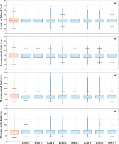
Figure 8. Spatial distribution of the rain gauges with 1 h average annual maxima higher than 50 mm (a). Location of the estimated values higher than 50 mm for Case 0 (b), Case 1 (c), Case 2 (d) and Case 5 (e).

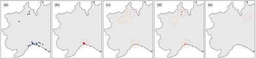
Figure 9. Slope coefficients of the regression models for the 1 h (a) and 24 h (b) duration in the case of r = 1 to 15 km.

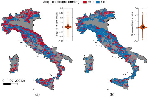
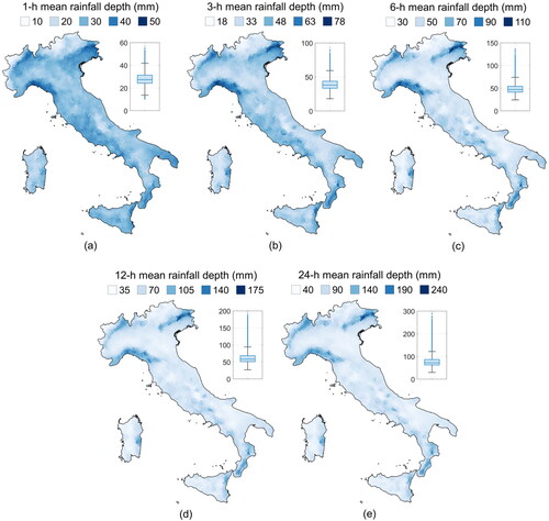
Figure 10. Average annual maxima for 1 (a), 3 (b), 6 (c), 12 (d) and 24 (e) hour intervals and related box plots.

Farr TG, Rosen PA, Caro E, Crippen R, Duren R, Hensley S, Kobrick M, Paller M, Rodriguez E, Roth L, et al. 2007. The shuttle radar topography mission. Rev Geophys. 45(2):RG2004.

 Web of Science ®Google Scholar

Data availability statement

Although Italian law requires an open-source policy for all public data, this right has not yet been implemented by all the Italian agencies involved in the management of the rain gauge network. The agreements we signed with some of these agencies, aimed at monitoring the correct use of the data, restricted their use to the aims of the authors’ project. As a result of these legal restrictions, a complete version of I²-RED can only be provided to two groups of people: members of the authors’ research group (who are already fully authorized to use the data) and people who can prove they have received clearance from the regional authorities. The entire quality-controlled database is available on Zenodo (https://doi.org/10.5281/zenodo.4269509), albeit with restricted access. The data can be used by third parties, for an indefinite timeframe, upon having completed an agreement with the authors and with the regional agencies involved in the data collection. The raw data availability depends on the region: a complete description of how to access these data is reported in Mazzoglio et al. (2020).