Multi-temporal InSAR and Sentinel-1 for assessing land surface movement of Joshimath town, India

Figures & data

Figure 1. Muddy water spurting out near J.P. Colony in Pekamarwadi area from a unknown source.

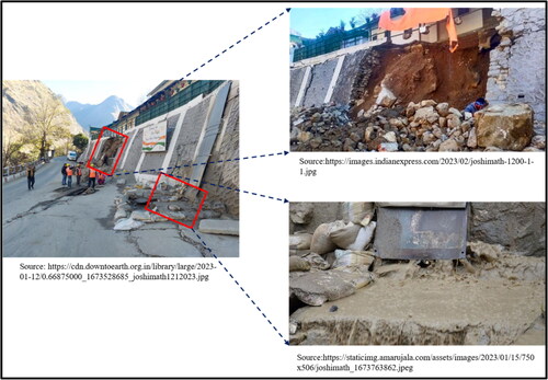
Figure 2. Field photographs of March–April 2022 – (a) building in Ravigram, (b) building in Lowerbazar, (c) community health centre building in Gandhinagar, (d) building in Pekamarwadi, (e-f) building in Singhdhar, (g) a subsided road section of NH-7 in Pekamarwadi, (h–i) road sections in Singhdhar.

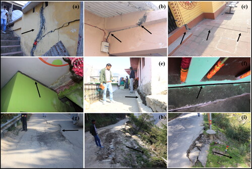
Figure 3. Location of study area – (a) map of Indian states and union territories, (b) districts map of Uttarakhand state, (c) administrative boundary of Chamoli district, and (d) wards map of Joshimath town.

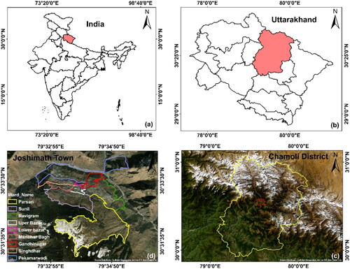
Figure 4. Small baseline network – (a) before modification, and (b) after coherence-based network modification. Lines in (a) and (b) represent interferograms coloured by average spatial coherence. Gray circle in (b) represents the excluded SAR acquisition.

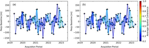
Figure 5. Methodological processing workflow of SBAS-InSAR time-series analysis. Gray ovals and rectangle represents steps in image domain; green and orange ovals and rectangle represent steps in interferogram domain; blue ovals and rectangles show the steps in time-series domain; white rhombi and green rectangle show input data; blue and white rectangles output data; dashed boundaries represents optional steps.

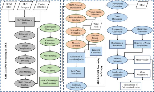
Table 1. Processing parameters used in different steps of MintPy processing.

Step	Method	Parameter	Used	Default
Modify_network	Coherence based	MinCoherence	0.22	0.7
Reference_point	Manual with high coherence	MinCoherence	0.80	0.85
		Spatial reference	30.574^0N, 79.56^0 E	NA
Correct_unwrap_error	Phase closure	NumSample	100	100
Invert_network	Weight function	Coherence	Coh	Var
		MaskThreshold	0.25	0.4
		MinRedundancy	1.0	1.0
		MinTempCoh	0.3	0.7
		MinNumPixel	100	100
Correct_troposphere	Height correlation	Looks	1	8
		PolyOrder	2	1
Deramp	Reliable pixels	Deramp	Quadratic	No
Correct_topography	Temporal deformation	PolyOrder	2	2
		StepFuncDate	No	No
Residual_RMS	Residual phase	Deramp	Quadratic	Quadratic
		Cut-off	3	3
Reference_date	Reference date	Date	20190505	20190505
Velocity	Velocity	Polynomial	1	1
		Periodic	1.0, 0.5	No
		StepDate	20230102	No
	Uncertainty	UncertaintyQuantification	Residue	Residue

Figure 6. Distribution of coherence – (a) average spatial coherence, and (b) temporal coherence.

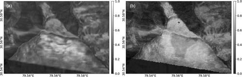
Figure 7. Inverted cumulative LOSD with temporal reference to 5 May 2019 – (a) raw LOSD, (b) SET corrected LOSD, (c) stratified tropospheric delay corrected LOSD, (d) De-ramped LOSD, (e) topographic residual corrected LOSD, and (f) RMS of residual displacement. The black circle and black plus sign represent the location of CORS station and spatial reference point, respectively.

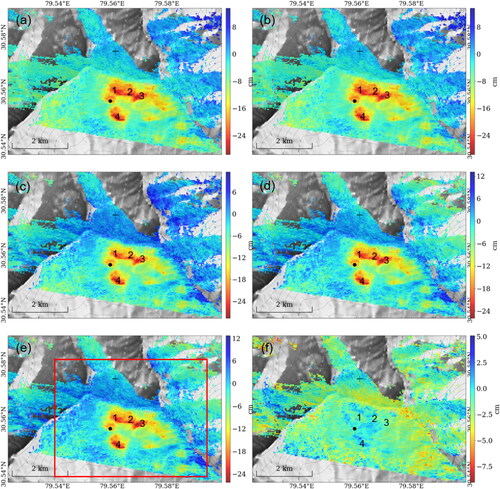
Figure 8. RMS value of residual phase for noise evaluation.

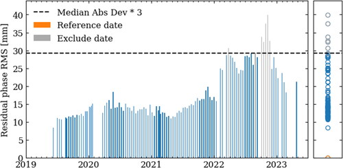
Figure 9. Correction of raw LOSD-TS at four point locations as shown in Figure 7.

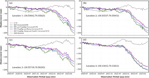
Figure 10. Cumulative LOS displacement overlaid with the wards boundaries. The black circle, plus sign and cross sign represents the locations of CORS station, spatial reference point and muddy water outlet, respectively.

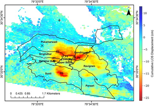
Figure 11. Cumulative LOS displacement time-series.

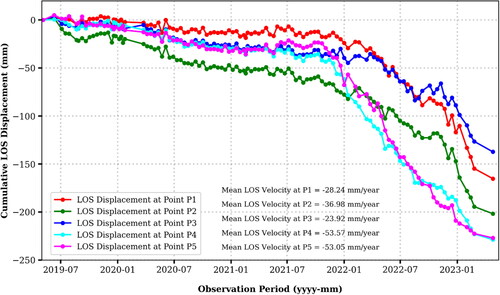
Figure 12. Velocity and acceleration and their standard deviations.

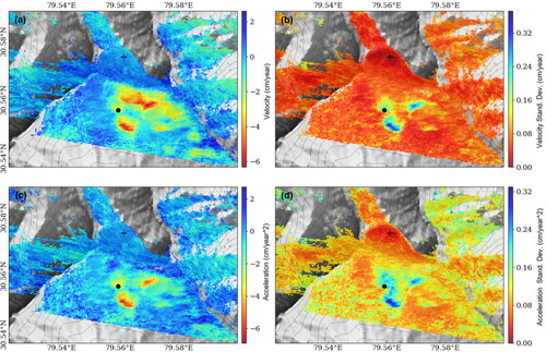
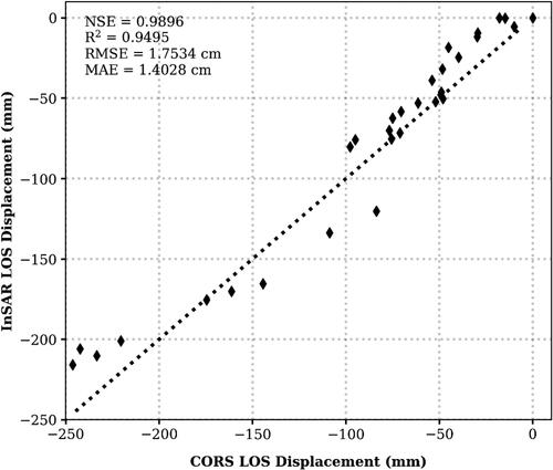
Figure 13. Comparison of SBAS-InSAR estimated and CORS derived LOSD.

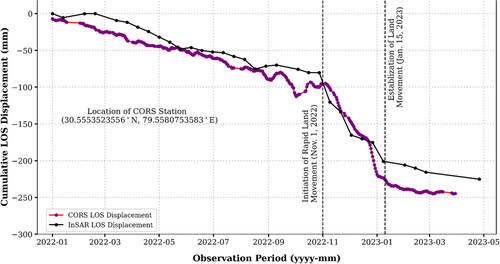
Figure 14. Accuracy assessment of SBAS-InSAR results at CORS location.