A novel model for multi-risk ranking of buildings at city level based on open data: the test site of Rome, Italy

Figures & data

Figure 1. Lithological units in the Municipality of Rome with the municipal districts, the study area, and the A90 highway outlined. Key to legend: 1: anthropic deposits; 3: recent and terraced sandy-gravelly alluvial deposits; 6: silty-sandy alluvial deposits, fluvio-lacustrine deposits; 7: travertines; 10: Plio-Pleistocene clayey and silty deposits; 11: marine Pliocene clays; 12: debris and talus slope deposits, conglomerates and cemented breccias; 14: marls, marly limestones and calcarenites; 41: leucitic/trachytic lavas; 43: lithoid tuffs, pomiceous ignimbritic and phreatomagmatic facies; 45: welded tuffs, tufites; 46: pozzolanic sequence; 55: alternance of loose and welded ignimbrites. EPSG:4326.

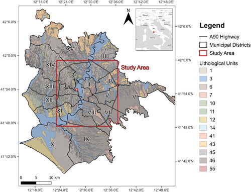
Figure 2. Flowchart of the adopted methodology to compute buildings’ single- and multi-risk scores. Coloured subplots report the workflow to derive the hazard (a), potential damage (b) and activity (c) components of the multi-risk equation. In bold the main inputs and outputs data.

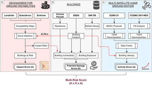
Table 1. Input data with features and role in the multi-risk ranking. ISTAT (istituto nazionale di STATistica) stands for ‘national institute of statistics’.

Input data	Description	Risk component	Format	Website/reference
Landslide susceptibility map	Spatial probability of landslides occurrence	Hazard	Raster (5 × 5m)	Esposito et al. (2023) Mastrantoni et al. (2023)
Subsidence susceptibility map	Spatial probability of subsidence occurrence	Hazard	Raster (5 × 5m)	Research contract CERI – ACEA ‘Development of a monitoring and prevention plan of the geo-hydrological instability of the city of Rome’
Sinkhole susceptibility map	Spatial probability of sinkhole occurrence	Hazard	Raster (5 × 5m)	Esposito et al. (2021), and Research contract CERI – ACEA.
ISTAT census tracts	Spatial distribution of building features	Vulnerability	Vector (polygons)	https://www.istat.it/
DBSN database	Building footprints and features	Building type and footprint	Vector (polygons)	https://www.igmi.org/
OMI database	Asset market value	Exposure	Vector (polygons)	https://www.agenziaentrate.gov.it/portale/
Sentinel-1 PS time series	Spatial distribution of ground motion rate	Activity	Vector (points)	https://land.copernicus.eu/pan-european/european-ground-motion-service
Cosmo-SkyMed PS time series	Spatial distribution of ground motion rate	Activity	Vector (points)	https://www.asi.it/en/earth-science/cosmo-skymed/
DTM	Elevation	Topography	Raster (5 × 5m)	Esposito et al. (2023)
ReNDiS	Mitigation Measures	Validation	Vector (points)	http://www.rendis.isprambiente.it/rendisweb/

Note: DBSN (DataBase di Sintesi Nazionale) stands for ‘national synthesis database’. OMI (Osservatorio Mercato Immobiliare) stands for ‘real estate market observatory’. ReNDiS (repertorio Nazionale degli interventi per la difesa del suolo) stands for ‘national inventory of soil protection interventions.

Figure 3. Susceptibility map for landslides (a), sinkholes (b) and subsidence (c) within the area of interest (AOI).

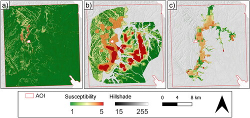
Table 2. Values of resistance factors employed in the structural resistance assessment (from Caleca et al. 2022).

Resistance factor	Parameter	Typology	Value
Structure type	ɛsty	Productive and commercial	0.1
		Residential with light structure	0.2
		Residential with brick walls	0.8
		Residential reinforced concrete	1.5
Maintenance state	ɛsmn	Productive and commercial	0.1
		Residential in very poor condition	0.1
		Residential in a medium condition	0.6
		Residential in a good condition	1.2
		Residential in a very good condition	1.5
Number of floors	ɛsht	Productive and commercial	0.1
		Single-storey residential	0.1
		Two-storey residential	0.4
		Three-storey residential	0.9
		Number of floors ≥4	1.5

Table 3. Contingency matrix for the assessment of building vulnerability by means of impact ratio and structural resistance classes (modified from Caleca et al. 2022).

Resistance	Impact ratio
	I0	I1	I2	I3	I4
R4	0	0	0.25	0.25	0.50
R3	0	0.25	0.25	0.50	0.50
R2	0	0.25	0.50	0.50	0.75
R1	0	0.25	0.50	0.75	0.75
R0	0	0.25	0.75	0.75	1
N.A.	0	0	0	0	0

Figure 4. PSs map of average velocity along LOS computed from long-term trends extracted from Sentinel-1 and Cosmo-SkyMed for ascending and descending orbits. EPSG:3857.

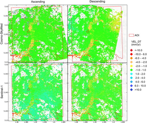
Figure 5. Overall number of buildings exposed (true) and unexposed (false) for each type of hazard investigated.

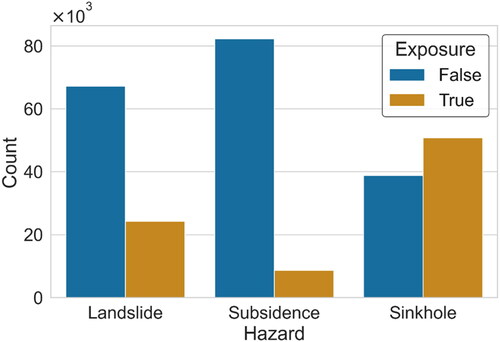
Figure 6. Hazard score of buildings for landslides (a), subsidence (b), and sinkholes (c). Statistical distribution of hazard score for elements at risk by hazard type (d). EPSG:3857.

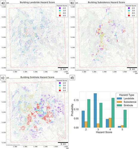
Figure 7. Probability density functions of impact ratio values by hazard type (a), and of structural resistance values for residential buildings.

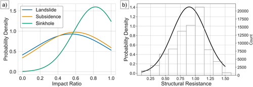
Figure 8. Graphical representation of the vulnerability value (V) assignment based on the contingency matrix reported in Table 3 (a). Distribution of vulnerability value of elements at risk by hazard type (b).

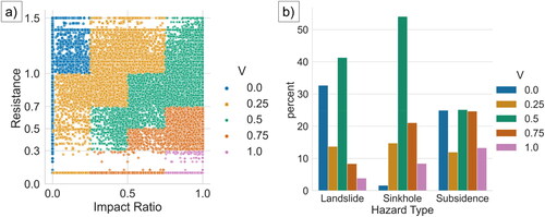
Figure 9. Real estate market values of buildings per square metre (€/m²) within the study area according to their category of use and position. EPSG:3857.

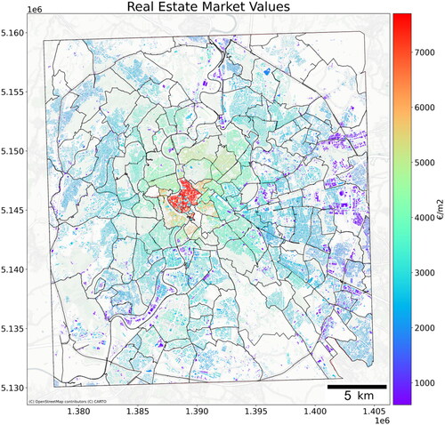
Figure 10. Potential damage score of buildings for landslides (a), subsidence (b), and sinkholes (c). Empirical cumulative distribution of economic losses per square metre selected according to hazard type (d). The coloured diamonds define percentile thresholds used to derive the five score classes. EPSG:3857.

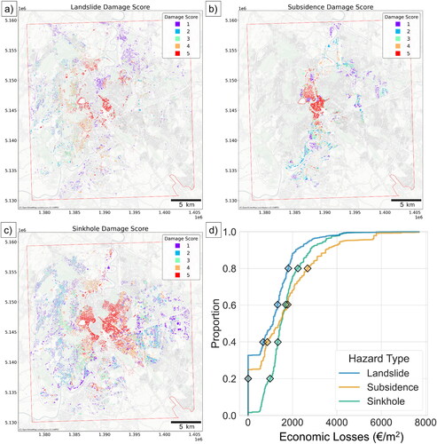
Figure 11. Buildings’ vertical (a) and horizontal (b) displacement rates (i.e. velocity) derived from the grid-based synthetic datasets (Figure A2) and assigned to the entire built-environment under investigation. EPSG:4326.

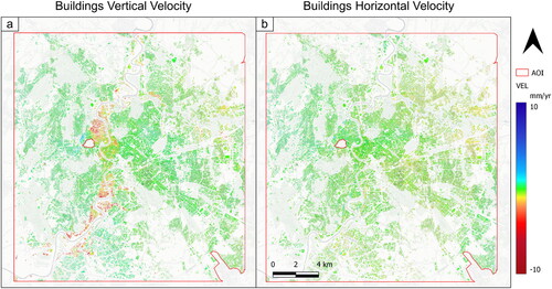
Figure 12. Activity score of buildings for landslides (a), subsidence (b), and sinkholes (c). Empirical cumulative distribution of absolute velocities values selected according to hazard type (d) employed to set up class thresholds. EPSG:3857.

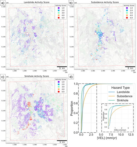
Figure 13. Risk score of buildings for landslides (a), subsidence (b), sinkholes (c) and multi-hazard (d).

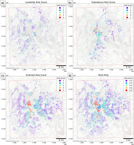
Figure 14. Spatial distribution of dominant risk threatening individual buildings (a) with a focus on the hazard type ratio among the overall elements (b), and among the buildings use categories (c).

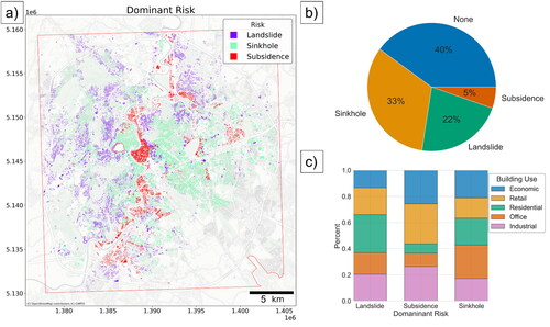
Figure 15. Average expenses (M€) and standard deviations of incurred mitigation measures within the study area compared with the multi-risk score of nearby buildings as computed in this work.

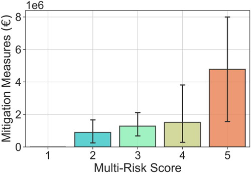
Figure 16. Ranking of the top 10 buildings with the highest absolute risk within the study area.

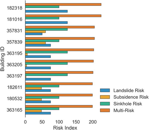
Figure A1. OMI macro-zones (a) and distribution of real-estate market values of buildings in Rome according to category of use and zone.

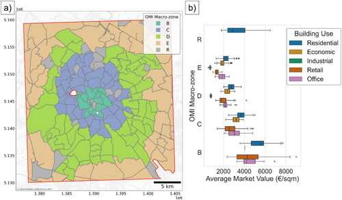
Figure A2. Synthetic datasets of up-down (a) and East-West (b) ground displacement rates derived from the data fusion of PSs resulting from A-DInSAR analyses of S1 and CSK SAR images.

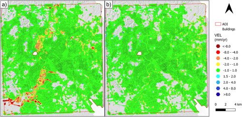
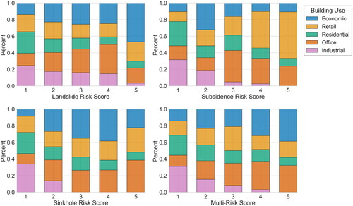
Figure A3. Distribution of building use categories according to single- and multi-risk scores.

Esposito C, Mastrantoni G, Marmoni GM, Antonielli B, Caprari P, Pica A, Schilirò L, Mazzanti P, Bozzano F. 2023. From theory to practice: optimisation of available information for landslide hazard assessment in Rome relying on official, fragmented data sources. Landslides. 20[(10):2055–2073. doi: 10.1007/s10346-023-02095-7.

 Web of Science ®Google Scholar

Mastrantoni G, Marmoni GM, Esposito C, Bozzano F, Scarascia Mugnozza G, Mazzanti P. 2023. Reliability assessment of open-source multiscale landslide susceptibility maps and effects of their fusion. Georisk. 0(0):1–18. doi: 10.1080/17499518.2023.2251139.

 Google Scholar

Esposito C, Belcecchi N, Bozzano F, Brunetti A, Marmoni GM, Mazzanti P, Romeo S, Cammillozzi F, Cecchini G, Spizzirri M. 2021. Integration of satellite-based A-DInSAR and geological modeling supporting the prevention from anthropogenic sinkholes: a case study in the urban area of Rome. Geomatics Nat Hazards Risk. 12(1):2835–2864. doi: 10.1080/19475705.2021.1978562.

 Web of Science ®Google Scholar

Caleca F, Tofani V, Segoni S, Raspini F, Rosi A, Natali M, Catani F, Casagli N. 2022. A methodological approach of QRA for slow-moving landslides at a regional scale. Landslides. 19(7):1539–1561. doi: 10.1007/s10346-022-01875-x.

 PubMed Web of Science ®Google Scholar

Data availability statement

All input data and the code are accessible online at the author’s GitHub page (https://github.com/gmastrantoni/mhr).