Investigating kinematics and triggers of slow-moving reservoir landslide using an improved MT-InSAR method

Figures & data

Figure 1. (a) Location of Xinpu landslide complex and coverage of the Sentinel-1 data used (black box), superimposed on the shaded relief map. The Xinpu landslide complex (red star) lies between two major counties (red dots), namely, Fengjie and yunyang. The inset is a sketch map of China. (b) Google Earth image of the Xinpu landslide complex, composed of the XiaErTai (XET) slope (including the submerged area shown as the orange dashed line), ShangErTai (SET) slope, and DaPing (DP) slope. The squares and triangles indicate the locations of GNSS stations and photos in Figure S1, respectively. Landslide outlines are from field survey.

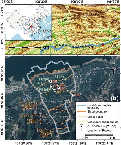
Figure 2. Geological setting of the Xinpu landslide complex. (a) Lithologic map with a scale of 1:500,000 showing the geological setting of the surrounding areas (J₁, J₂, J₃: Lower, Middle, and Upper Jurassic strata; T₁, T₂, T₃: Lower, Middle, and Upper Triassic strata; the red region is the study area). (b) Geological plane map of the Xinpu landslide complex. (c) a longitudinal cross-section G-G’ of XET slope showing the inferred limits of different subzones.

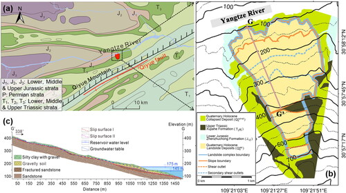
Figure 3. Flowchart of the implemented method.

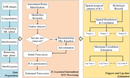
Figure 4. Spatial and temporal baselines of the generated interferometric pairs from 124 Sentinel-1 scenes.

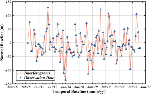
Figure 5. Spatial–temporal pattern of the Xinpu landslide complex. (a) LOS deformation rate field derived using our method. The background is a three-dimensional model derived from SRTM DEM. (b–c) Time-series accumulative displacements (colorful lines) and elevation (gray areas) along (b) P–P′, (c) a–a′, and (d) B–B′ profiles.

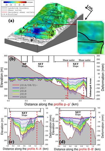
Figure 6. Photos from the field investigation. (a) Mini kinematic unit, which is observed in the derived spatial pattern. (b & c) The secondary shear outlets of L1 and L2 in Figure 5(a).

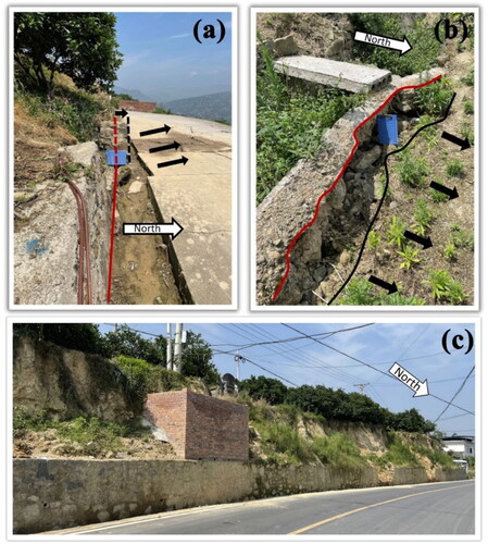
Figure 7. LOS time series accumulative deformation is measured at the G3 (the red triangle) and G5 (the blue inverted triangle) stations. The location of G3 and G5 can be found in Figure 1. The gray areas indicate the wet season of each year.

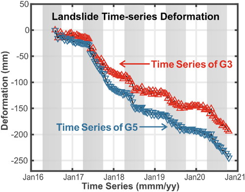
Figure 8. (a) Cumulative deformations along the secondary shear outlet. (b) Corresponding location of the section with strong deformation. The background is a Google Earth image.

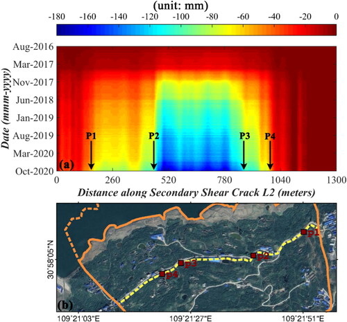
Figure 9. Contribution of (a) IC4 and (b) IC5 derived by ICA. Comparisons between precipitation (green triangle), water level (blue areas), and normalized IC eigenvectors of (c) IC4 and (d) IC5. (e) & (f) Relationship between correlation and lag time for corresponding triggers.

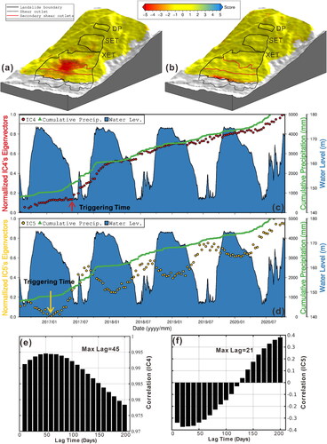
Figure 10. Results of synthetic datasets. (a) Simulation deformation rate. (b-e) Deformation rates derived by conventional SBAS, ISBAS, and our method, respectively. (f-i) Residuals of the corresponding methods in the second row.

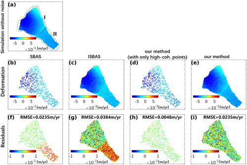
Figure 11. Annual rate of movements derived using different MT-InSAR techniques in the Xinpu landslide complex. (a) SBAS, (b) DSI, (c) our method before ICA optimization, and (d) our method after ICA optimization. The background image used is a Google Earth image.

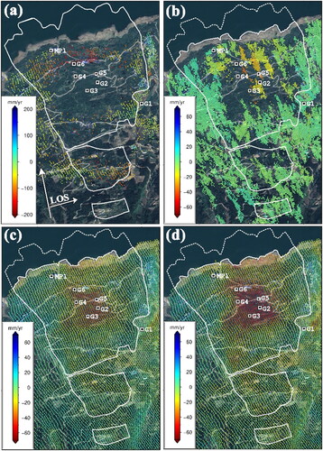
Figure 12. Landslide time-series deformation derived by DSI (orange square), our method (before and after ICA optimization, shown with blue inverted triangle and red triangle, respectively), and GNSS observations (green asterisk) in (a) G2 (b) G3, (c) G4, (d) G5, and (e) G6 GNSS monitoring stations. The gray areas indicate the wet season of each year. (f) The time-series movements derived by various MT-InSAR methods.

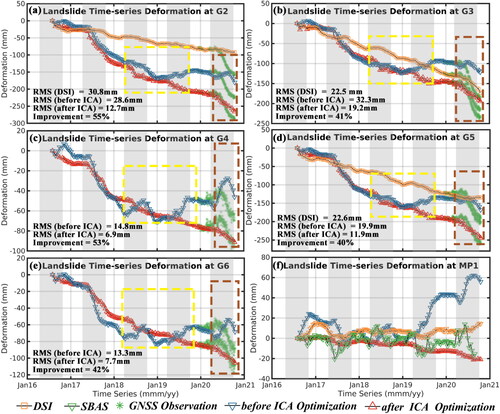
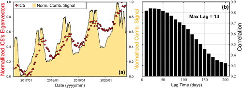
Figure 13. (a) Comparison between IC5 (red dot) and the normalized combined signal (yellow areas) after combining the precipitation and water level records. (b) Relationship between correlation and lag time.

Data availability statement

The Sentinel-1 data were provided by ESA/Copernicus (https://scihub.copernicus.eu/). Other datasets used to support the findings of this study are available from the corresponding author upon request.