
Figures & data
Figure 1. Yellow stars show the spatial distribution of boulder deposits around the Mediterranean Sea (modified from Mottershead et al. Citation2018). most of these deposits are reportedly of mixed origin (i.e. storm and tsunami). the red dots indicate the boulder accumulations recently discovered in north Croatia (Biolchi et al. Citation2019a,Citationb).
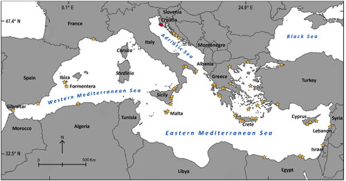
Figure 2. (a) Location of the Istrian peninsula and Fenoliga Island; (b) the longest fetch distance associated with the sirocco; (c) wind frequency averaged over 30 years (www.meteoblue.com); (d) wave frequency for north Adriatic (Katalinić and Parunov Citation2021); and (e) geological map of the Istrian Peninsula (derived from geological map of Croatia in scale 1:300.000 produced by hrvatski geološki institut (Citation2009)).
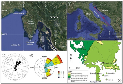
Figure 3. (a) Landsat image of Fenoliga Island (Google Earth, 2022); (b) oblique view of the sloping coastal profile taken in the southern part of the island where the boulders are most abundant.
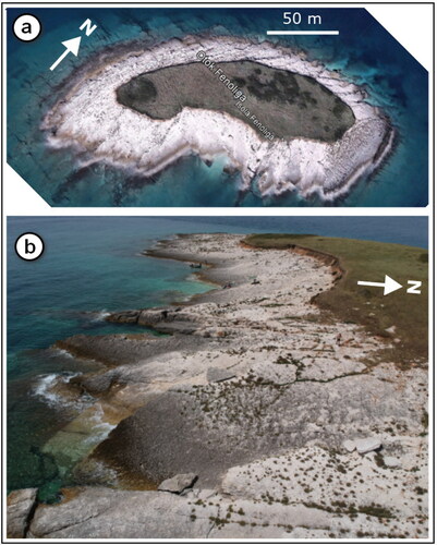
Table 1. Main characteristics of the DJI SparkTM.
Table 2. Coordinates of GCPs (WGS 84/UTM zone 33 N (EPSG:32633).
Figure 4. Processing workflow using Metashape for the creation of the virtual study area model. (a) Photos were captured by three UAV flights and were later imported into Metashape for SfM-MVS processing. (b) The result of the photo alignment was a sparce point cloud that, (c) after the inclusion of the 4 GCPs was (d) densified. (e) The mesh was obtained from the filtered dense cloud and, (f) textured. A magnification of the textured mesh depicting a GCP is shown. (g) The DEM; and, (h) the orthomosaic used in GIS.
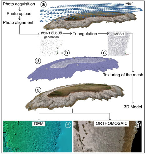
Table 3. Coordinate error of GCPs. In the last column in brackets are indicated the number of projections of the GCPs.
Table 4. Attributes of the ESRI shapefile named ‘boulders_calc_b_axis’.
Figure 5. The spatial distribution of coastal boulders (white polygons), the red arrow indicates the largest boulder on the island (b-axis length is 4.81 m).
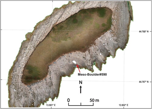
Figure 6. QGIS representation of boulder dataset analysis. (a) Spatial distribution of boulders according to size (Terry and Goff Citation2014); (b) minimum distance of the boulders from the coastline.
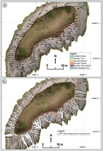
Table 5. Boulder size analysis based on the nomenclature proposed by Terry and Goff (Citation2014).
Figure 7. The image depicts the digitized, and numbered, detached boulders located on the rocky foreshore of Fenoliga Island using Google Earth, Landsat imagery from February 2, 2013.
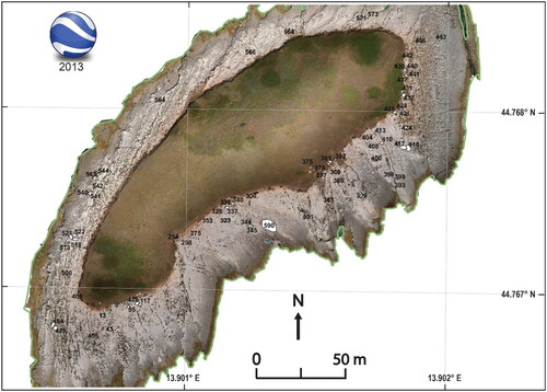
Figure 8. (a) map view of boulder movements for the period 2013-2022 comparing the position using Google Earth imagery (February 2, 2013), and the UAV-derived orthomosaic (June 27, 2022); (b) view of boulder displacement #344, #345, and #590; (c) view of boulder displacement #417, and #418.
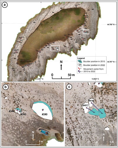
Table 6. List of the five boulders that have undergone the greatest displacement during the period February 2, 2013 to June 27, 2022.
Figure 9. (a) Fractures and bedding mapped from the 3D model; (b) lower hemisphere, stereographic equal-area projections of poles to fractures (green dots) and to bedding (yellow squares) and associated contour plot after data filtering based on vertex collinearity (Woodcock Citation1977; Fernández Citation2005; Seers and Hodgetts Citation2016); (c) half-range rose diagram showing the distribution of the fracture strikes with the highlight of the main angles formed between the main fracture sets; and, (d) detail of selected boulders showing that angularity follows the dihedral angles of the fracture sets mapped in the 3D model of the island.
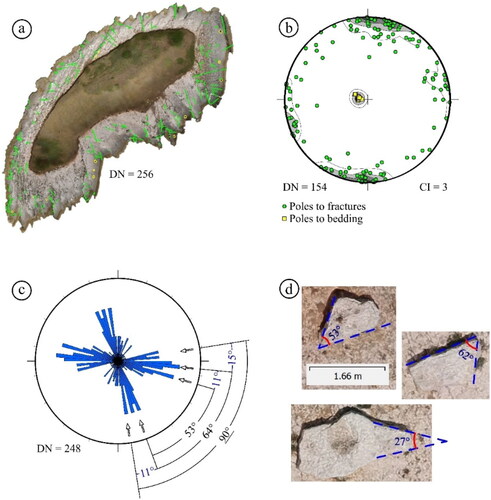
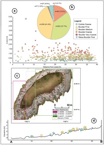
Figure 10. (a) Pie chart showing the percentages of boulder size by sedimentary classification; (b) scatter plot diagram showing boulder size (b-axis) relative to the recorded distance from the coastline; (c) distribution of boulders classified according to longitude; (d) topographic profile (A - B) approximately normal to the coastline.
Data availability statement
Datasets used in this study are available via: doi.org/10.6084/m9.figshare.24057843.v1.