
Figures & data
Figure 1. General structure of a convolutional neural network.
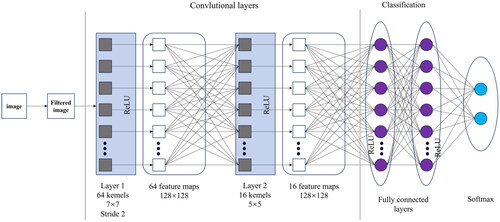
Figure 2. Schematic diagram of the DenseLayer.
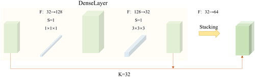
Figure 3. DenseNet architecture connectivity.
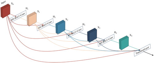
Figure 4. Schematic diagram of group convolution.
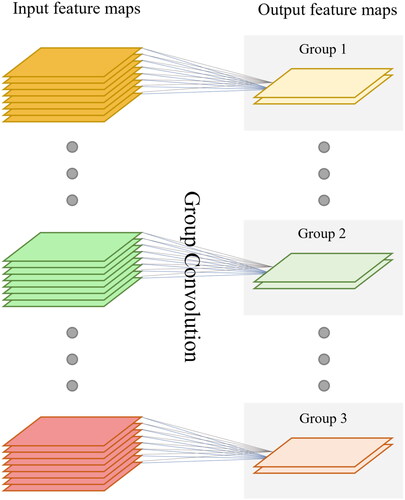
Figure 5. Squeeze and excitation module illustration.
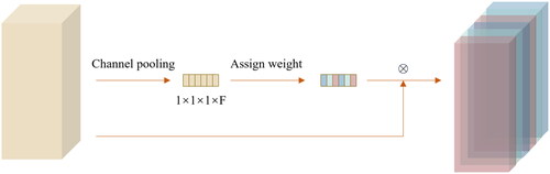
Table 1. DenseNet + GC + SE network architecture.
Figure 6. Illustrates the DenseNet network architecture and the data transmission process.
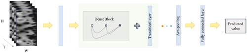
Figure 7. Schematic layout of the experimental setup with acoustic emission sensors.
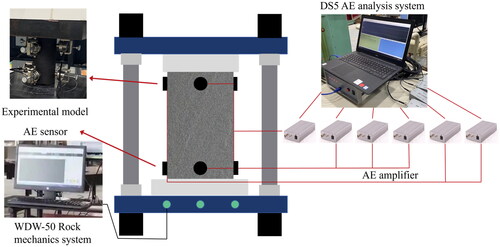
Table 2. Physical and mechanical parameters of the sample and loading rate.
Figure 8. Uniaxial compression experimental results.
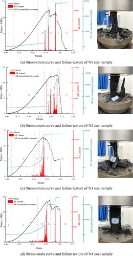
Figure 9. Acoustic emission waveforms at different stages. (a) Stage one (b) stage two (c) stage three (d) stage four (e) stage five (f) stage six.
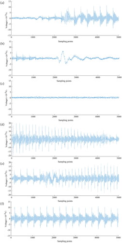
Figure 10. Waveform after wavelet transform of acoustic emission. (a) Stage one (b) stage two (c) stage three (d) stage four (e) stage five (f) stage six.

Table 3. YOLO model performance comparison table.
Figure 11. YOLOv5 algorithm performance test for each version.
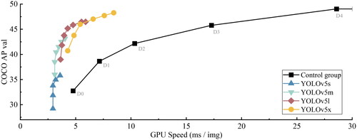
Figure 12. YOLOv5s structure diagram.
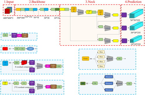
Table 4. Model training parameters.
Table 5. Validation set training results.
Figure 13. Training/validation set – accuracy and cross-entropy loss.
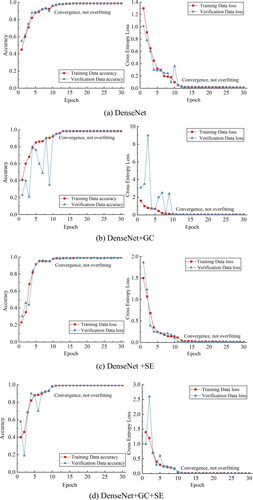
Figure 14. Probability distribution of output for validation samples.
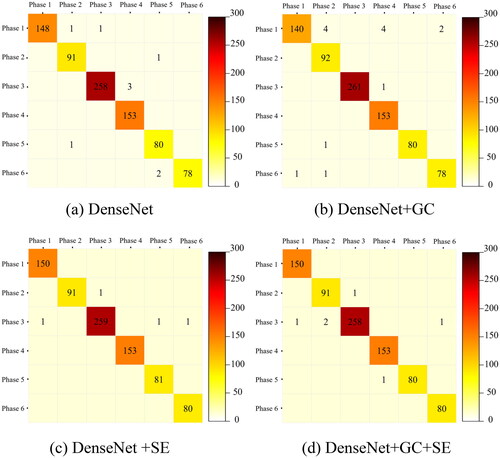
Figure 15. The utility of group convolution in characterizing the diversity of acoustic emission features.
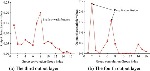
Figure 16. The utility of the SE module – representing the importance of acoustic emission features.
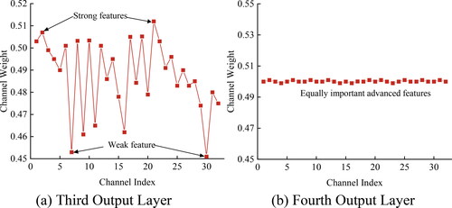
Table 6. Comparison of different 3D network performances.
Data availability statement
All the data, models or code generated or used in the present study are available from the corresponding author by request.