
Figures & data
Figure 1. CDF curves of the model climatological and ensemble forecast.
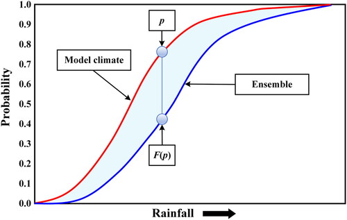
Figure 2. Illustration of the stacking ensemble learning framework.
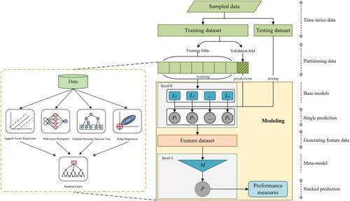
Figure 3. Flowchart of the proposed stacking ensemble learning strategy.
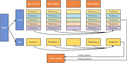
Figure 4. Flowchart of the PSO-ML model for hyperparameter optimization.
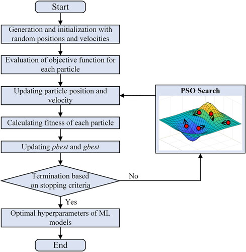
Table 1. Model hyperparameter setting.
Table 2. The characteristics of acceptable results for RPE, RMSE, MAE, and NSE.
Figure 5. Sub-area divisions in the study area.
Figure 6. Daily inflow of the Geheyan Reservoir.
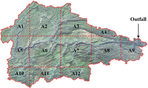
Figure 7. Daily inflow of the Geheyan Reservoir.
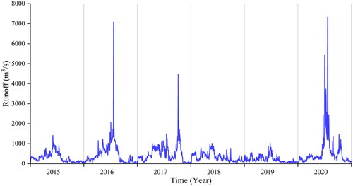
Figure 8. Monthly runoff ratio of the total annual runoff.
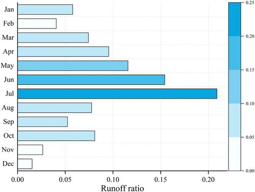
Table 3. Summary of the training dataset (count = 460).
Table 4. Summary of the testing dataset (count = 92).
Figure 9. EFI values of 12 sub-areas with different lead times.
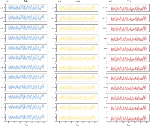
Figure 10. Importance measures with different lead times.
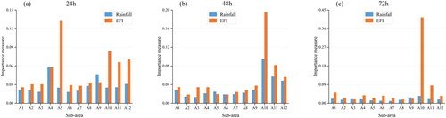
Table 5. Optimal PSO-ML hyperparameters for different lead times in rainfall-runoff simulation.
Table 6. Optimal PSO-ML hyperparameters for different lead times in EFI-runoff simulation.
Figure 11. Rainfall, EFI, and runoff time series on the held-out testing samples with different lead times.
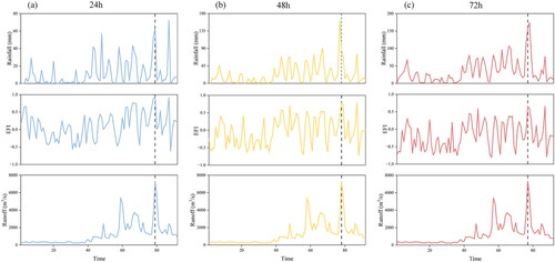
Figure 12. Multiple model prediction results on the held-out testing samples obtained by two inputs with different lead times.
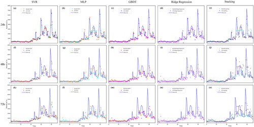
Table 7. Evaluation indices comparison of two inputs.
Figure 13. Comparisons of multiple model prediction results on the held-out testing samples with different lead times.
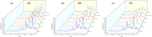
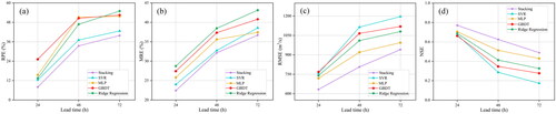
Figure 14. Four evaluation indices of the predictions using the SVR, BP, GBDT, Ridge Regression, and stacking model for different lead times.
Data availability statement
Data will be made available on request.