
Figures & data
Figure 1. Study area and historical landslide distribution:(a) Gansu in China, (b)study area in Gansu province, (c) historical landslides, (d) the google image and landslide boundary of North Hill landslide, (e) the field photograph of North Hill landslide, (f) the google image and landslide boundary of Jiangdingya landslide, (g) the field photograph of Jiangdingya landslide.
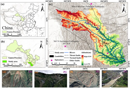
Figure 2. The spatial distribution of LIFs: (a) altitude, (b) slope, (c) profile curvature, (d) TWI, (e) rainfall, (f) land use, (g) NDVI, (h) lithology, (i) soil type, (j) distance to roads, (k) distance to Rivers, (l) distance to faults.
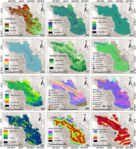
Table 1. The sources of data for LIFs used in this study.
Figure 3. Flow chart of this study.
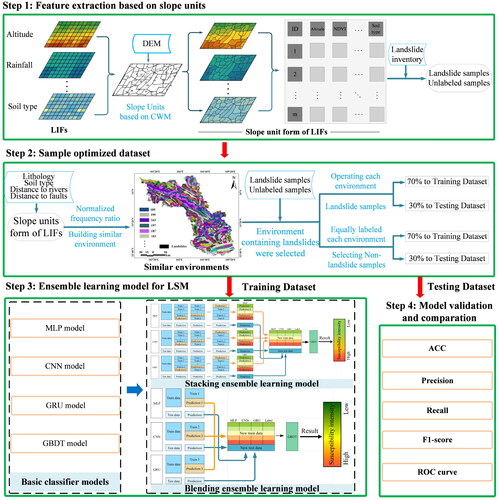
Figure 4. Flowcharts of slope unit generation.
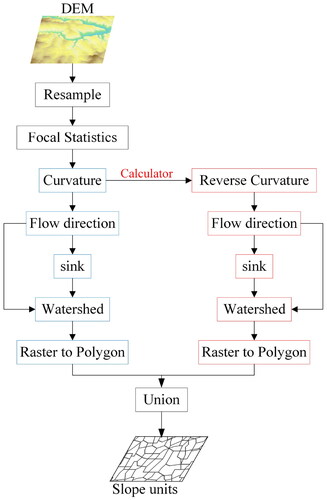
Figure 5. Classes and weights of disaster-pregnant environment factors.
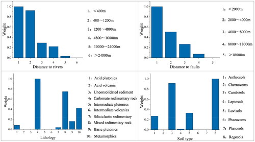
Figure 6. (a) The spatial distribution of similar environments. (b) The number of landslide samples distributed in each environment.
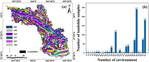
Figure 7. Distribution of sample sites: (a) non-landslide samples based on SEM, (b) non-landslide samples based on RM.
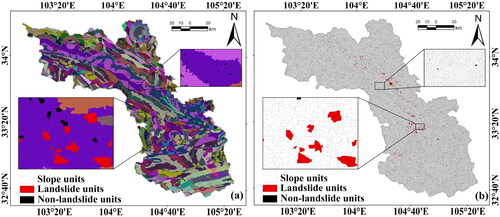
Figure 8. The structure of MLP model.
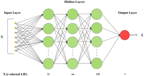
Figure 9. The structure of CNN model.
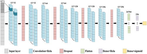
Figure 10. The structure of GRU model.
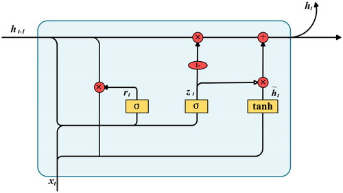
Figure 11. The structure of stacking ensemble learning model.
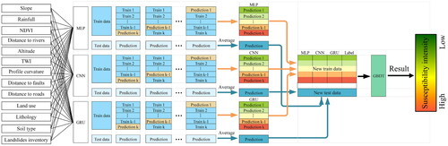
Figure 12. The structure of blending ensemble learning model.
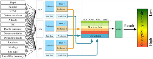
Figure 13. (a) Multicollinearity evaluation of LIFs. (b) Variable importance of each LIF using random Forest.
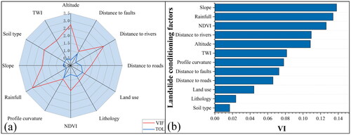
Table 2. Relationship between the historical landslides and LIFs.
Figure 14. LSMs Generated using (a) stacking based on the RM, (b) blending based on the RM, (c) stacking based on the SEM, and (d) blending based on the SEM. Regions A and B are zoomed in to provide an intuitive visualization of LSM using different non-landslide sampling methods. The lowest subfigure shows the proportion of area at each landslide susceptibility level.
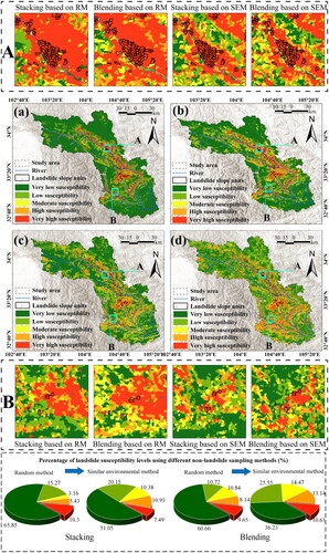
Table 3. Accurate metrics for ensemble models using different testing dataset.
Figure 15. The distribution of samples in each class of altitude.
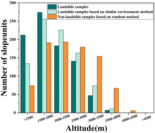
Figure 16. (a) LSM generated using stacking based on RM, (b) LSM generated using blending based on RM, (c) field verification photograph, (d) Google earth image, (e) LSM generated using stacking based on SEM, (f) LSM generated using blending based on SEM.
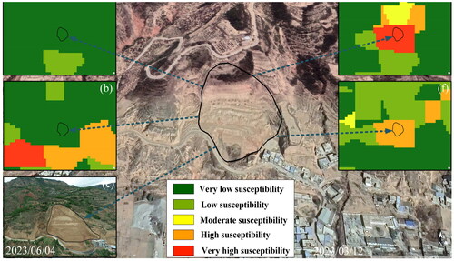
Figure 17. (a) LSM generated using stacking based on RM, (b) LSM generated using blending based on RM, (c) field verification photograph, (d) Google Earth image, (e) LSM generated using stacking based on SEM, (f) LSM generated using blending based on SEM.
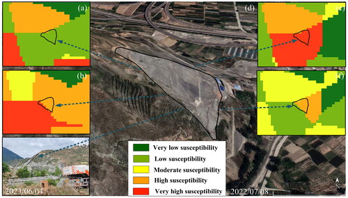
Figure 18. LSM generated using (a) MLP, (b) CNN, (c) GRU, (d) stacking and (e) blending.
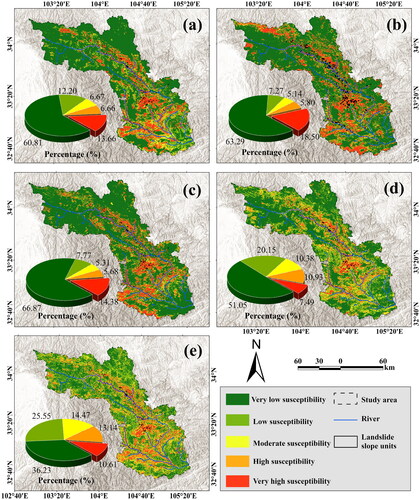
Figure 19. ROC curves of different models using testing dataset.
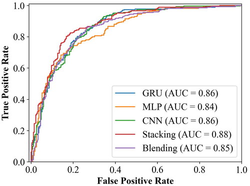
Figure 20. FR values for the levels of landslide susceptibility across different models.
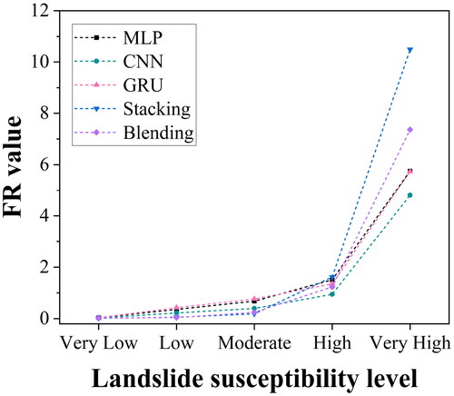
Table 4. Accurate metrics for each model using testing dataset based on SEM.
Data availability statement
The datasets used or analysed during this study are available from the corresponding author on reasonable request.