Classification of hyperspectral data using extended attribute profiles based on supervised and unsupervised feature extraction techniques

Figures & data

Figure 1. The work flow of spectral-spatial classification with EMAP. The dotted lines indicate the possibility of switching between supervised and unsupervised feature reduction. An optional feature reduction step can be used to reduce the dimensionality of EMAP before classification.

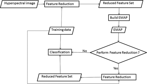
Figure 2. Indian Pine dataset. (a) False colour representation of the Indian Pines image, (b) test and (c) training sets.

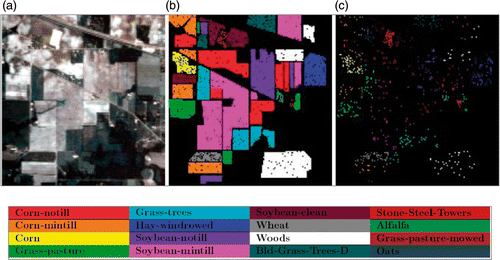
Table 1. Number of training and test pixels used for the Indian Pines image.

Class	Training	Test
Corn-notill	50	1384
Corn-mintill	50	784
Corn	50	184
Grass-pasture	50	447
Grass-trees	50	697
Hay-windrowed	50	439
Soybean-notill	50	918
Soybean-mintill	50	2418
Soybean-clean	50	564
Wheat	50	162
Woods	50	1244
Bld-grass-trees-D	50	330
Stone-steel-towers	50	45
Alfalfa	15	39
Grass-pasture-mowed	15	11
Oats	15	5

Figure 3. Pavia University dataset. (a) False-colour representation of the University of Pavia image, (b) test and (c) training set.

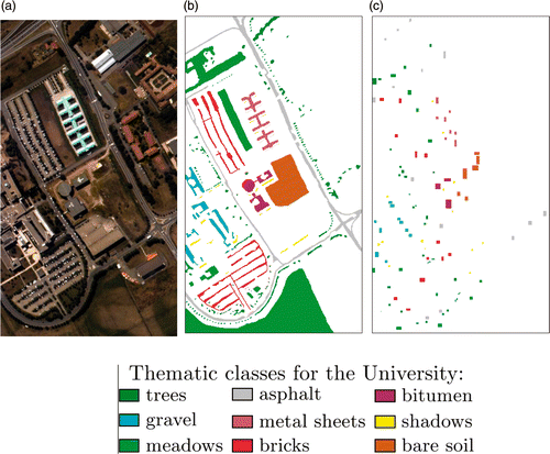
Table 2. Number of training and test pixels used for the Pavia image.

Class	Training	Test
Trees	524	2912
Asphalt	548	6304
Bitumen	375	981
Gravel	392	1815
Metal sheets	265	1113
Shadow	231	795
Bricks	514	3364
Meadows	540	18,146
Bare soil	532	4572

Table 3. Accuracies (%) for classification of Indian Pines image. The best results in terms of accuracy are marked in bold.

Panel A: Results using RF with spectral information only
Cass	Spectral	PCA	KPCA	DAFE	DBFE	NWFE
Features	220	10	25	15	20	20
1	51.16	56.65	55.27	52.96	49.13	75.22
2	51.28	66.84	73.21	52.17	47.96	63.9
3	81.52	72.83	86.41	78.26	70.11	84.24
4	88.81	91.50	93.74	84.12	79.64	92.39
5	82.50	87.66	83.36	88.38	89.24	92.54
6	90.21	96.58	92.48	98.18	98.63	98.86
7	69.28	62.09	77.78	60.46	62.31	81.26
8	51.24	58.44	59.76	38.96	42.68	56.53
9	65.60	74.29	72.16	65.96	68.09	78.19
10	93.83	97.53	98.15	97.53	98.77	99.38
11	81.27	90.27	88.5	84.81	85.05	93.41
12	70.00	67.27	73.03	82.12	70.00	74.24
13	95.56	100	100	97.78	93.33	97.78
14	56.41	87.18	82.05	53.85	48.72	76.92
15	72.73	90.91	90.91	100	81.82	100
16	80.00	100	100	40.00	20.00	100
AA	73.83	81.25	82.93	73.47	69.09	85.30
OA	65.59	71.19	73.03	63.49	63.12	76.53
κ	61.33	67.46	69.63	59.00	58.50	73.50
Panel B: Results of RF with profiles
Class	PCA p	KPCA p	DAFE p	DBFE p	NWFE p	NW-NW	KP-NW
Features	130	325	195	260	260	30	30
1	82.23	89.88	77.75	77.46	91.04	88.44	80.20
2	95.15	97.70	85.71	83.93	98.21	94.01	93.37
3	96.74	96.74	91.30	86.41	97.83	90.22	95.65
4	94.18	94.41	93.96	92.17	93.96	93.74	94.41
5	98.71	98.42	97.42	97.99	99.71	96.99	98.57
6	99.54	99.54	99.77	100	100	99.54	98.63
7	89.87	86.71	75.27	88.13	88.67	82.03	78.21
8	91.27	93.92	72.42	82.09	93.22	89.62	91.11
9	92.38	95.74	79.96	85.28	95.21	92.73	90.25
10	99.38	99.38	98.77	99.38	99.38	99.38	99.38
11	99.44	99.76	98.63	94.94	99.52	90.51	93.41
12	97.27	98.48	98.18	90.00	98.79	95.76	99.09
13	100	100	100	100	100	100	100
14	94.87	92.31	97.44	97.44	97.44	94.87	97.44
15	100	100	100	100	100	100	100
16	100	100	100	80.00	100	100	100
AA	95.69	96.44	91.66	90.95	97.06	94.24	94.36
OA	92.83	94.76	84.33	87.22	95.06	91.03	90.36
κ	91.80	93.40	82.20	85.43	94.34	89.75	89.00
Panel C: Results using SVM with spectral information only
Class	Spect.	PCA	KPCA	DAFE	DBFE	NWFE
Features	220	10	25	15	20	20
1	53.47	62.21	66.04	47.76	50.29	66.55
2	58.16	65.31	75.64	43.88	47.58	53.57
3	78.80	84.78	83.15	75.54	75.54	78.80
4	85.68	89.04	94.85	87.47	84.34	89.93
5	80.20	90.96	90.82	84.51	86.08	90.96
6	94.99	93.39	94.76	98.18	96.58	98.18
7	78.43	65.69	79.85	58.50	62.64	72.88
8	59.51	55.67	64.52	43.88	47.68	46.86
9	61.52	68.26	77.48	64.18	67.55	79.26
10	95.68	98.15	98.77	99.38	99.38	99.38
11	90.27	93.49	90.03	84.41	85.21	84.73
12	54.24	62.42	72.42	82.12	78.18	75.15
13	97.78	95.56	97.78	93.33	93.33	95.56
14	51.28	76.92	92.31	43.59	64.10	74.36
15	81.82	81.82	90.91	72.73	90.91	81.82
16	100	100	100	20.00	40.00	60.00
AA	76.36	80.23	85.58	68.72	73.09	78.00
OA	69.70	71.55	77.31	62.71	64.90	69.79
κ	65.76	67.87	74.3	57.97	60.32	66.03
Panel D: Results using SVM with profiles
Class	PCA p	KPCA p	DAFE p	DBFE p	NWFE p	NW-NW	KP-NW
Features	130	325	195	260	260	30	30
1	72.47	79.41	58.09	66.91	79.62	90.24	84.03
2	87.37	92.73	58.67	76.28	79.34	98.85	98.21
3	91.85	96.20	83.70	84.78	83.15	97.28	98.91
4	91.28	93.96	93.29	92.62	93.29	95.52	97.54
5	98.42	98.42	86.51	94.84	95.55	99.56	98.85
6	98.63	98.63	94.76	98.41	99.32	99.54	99.32
7	79.96	87.36	67.97	75.16	78.32	86.27	89.11
8	83.83	87.84	56.00	65.47	65.55	94.58	93.71
9	84.22	86.35	69.68	81.21	88.83	93.61	87.41
10	99.38	99.38	96.91	99.38	99.38	99.38	99.38
11	94.86	95.90	87.46	89.71	92.36	92.76	98.63
12	94.24	96.36	95.15	91.52	95.15	99.09	99.09
13	100	100	82.22	97.78	97.78	100	100
14	92.31	94.87	30.77	79.49	79.49	94.87	97.44
15	100	90.91	18.18	63.64	100	100	100
16	100	100	20.00	60.00	100	100	100
AA	91.80	93.64	68.71	82.32	89.196	96.35	96.35
OA	86.53	90.20	70.69	78.39	81.853	94.17	93.75
κ	84.67	88.82	66.80	75.50	79.43	93.33	92.84

Table 4. Accuracies in percentage for classification of the University of Pavia image. The best results in terms of accuracy are marked in bold.

Panel A: Results using RF with spectral information only
Class	Spect.	PCA	KPCA	DAFE	DBFE	NWFE
Features	103	4	20	8	25	18
1	98.69	99.05	98.96	92.75	93.93	98.24
2	81.28	77.45	79.61	82.75	84.93	86.4
3	84.44	80.98	85.26	83.83	85.49	90
4	52.74	49.69	50.88	71.94	67.51	60.74
5	99.11	99.11	99.48	100	99.85	99.78
6	98.10	98.52	97.15	97.99	98.2	99.79
7	91.06	89.44	89.27	82.78	87.53	93.48
8	55.61	56.37	57.05	72.05	66.88	64.08
9	79.22	76.4	77.37	89.06	93.8	93.16
AA	82.25	80.78	81.67	85.91	86.46	87.3
OA	71.57	70.61	71.51	79.93	78.9	78.49
κ	65.07	63.82	64.89	74.63	73.62	73.26
Panel B: Results using RF with profiles
Class	PCA p	KPCA p	DAFE p	DBFE p	NWFE p	DB-DB	DA-DB	KP-DB
Features	68	340	136	425	306	26	30	30
1	99.15	99.90	92.36	96.93	99.44	94.97	98.82	99.08
2	94.86	96.54	95.86	97.60	96.83	96.54	95.62	96.57
3	99.70	99.84	100	99.32	99.77	100	99.92	99.84
4	67.56	94.33	88.32	81.41	66.46	74.51	74.41	76.13
5	99.63	99.77	99.85	99.85	99.70	100	100	99.70
6	99.79	99.89	96.30	99.89	100	98.52	99.26	96.93
7	99.02	99.80	99.51	98.47	99.45	99.37	98.39	99.67
8	96.48	94.04	98.08	96.72	97.72	98.53	80.54	87.39
9	73.28	64.44	88.06	90.87	61.10	97.31	89.99	78.76
AA	92.16	94.28	95.37	95.67	91.16	95.53	92.99	92.68
OA	92.76	92.37	95.87	95.83	92.19	96.81	88.16	90.13
κ	90.36	89.85	94.55	94.49	89.51	95.79	84.81	87.14
Panel C: Results using SVM with spectral information only
Class	Spect.	PCA	KPCA	DAFE	DBFE	NWFE
Features	103	4	20	8	25	18
1	97.98	97.68	98.56	86.88	94.75	90.21
2	84.35	70.25	79.49	79.16	81.77	82.23
3	91.88	85.56	89.32	83.76	86.47	87.37
4	71.37	55.93	63.41	66.84	71.37	71.13
5	99.33	98.44	99.48	99.78	99.63	99.78
6	97.99	94.4	94.93	99.16	98.2	98.84
7	92.69	86.34	89.84	80.74	84.95	89.35
8	70.44	58.05	69.7	67.83	66.79	64.1
9	93.64	72	85.54	87.87	91.85	94.43
AA	88.85	79.85	85.59	83.56	86.2	86.38
OA	81.44	69.68	78.68	76.56	78.19	77.48
κ	76.74	62.6	73.28	70.64	72.78	72
Panel D: Results using SVM with profiles
Class	PCA p	KPCA p	DAFE p	DBFE p	NWFE p	DB-DB	DA-DB	KP-DB
Features	68	340	136	425	306	26	30	30
1	98.73	99.64	97.09	94.97	96.93	95.43	98.53	96.96
2	92.34	94.11	93.15	92.84	92.14	95.88	94.98	95.27
3	99.70	99.24	99.92	98.05	97.07	100	99.92	99.77
4	61.03	92.28	79.99	68.84	82.71	90.94	76.46	90.13
5	99.48	99.62	99.33	99.93	99.93	100	100	99.77
6	89.23	99.15	96.62	96.09	97.25	98.41	98.31	99.36
7	99.16	99.40	97.12	94.84	97.28	99.18	98.78	98.26
8	96.14	89.70	98.36	89.38	82.13	98.65	91.93	88.20
9	92.36	78.16	99.44	98.83	97.77	99.96	97.30	87.73
AA	92.02	94.59	95.67	92.64	93.69	97.60	95.13	95.05
OA	93.89	91.52	96.62	91.64	89.27	97.89	93.98	91.80
κ	91.95	88.92	95.55	89.14	86.24	97.22	92.14	89.34

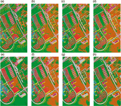
Figure 4. Classification maps for Indian Pines data with RF classifier using (a) Original data (b) PCA, (c) KPCA, (d) DAFE, (e) DBFE and (f) NWFE.

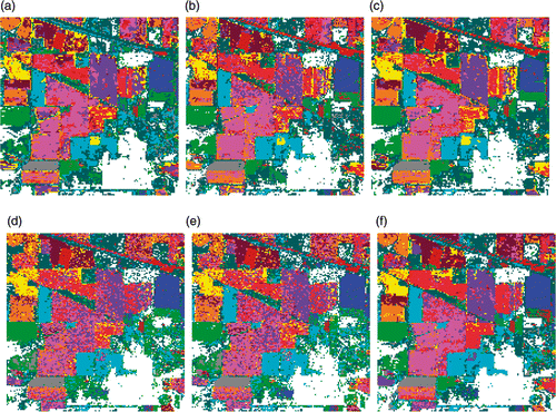
Figure 5. Classification maps for Indian Pines data with SVM classifier using (a) Original data (b) PCA, (c) KPCA, (d) DAFE, (e) DBFE and (f) NWFE.

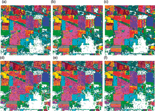
Figure 6. Classification maps for Indian Pines data with RF classifier using EMAPs of (a) PCA, (b) KPCA, (c) DAFE, (d) DBFE and (e) NWFE, and feature reduction applied on EMAP using (f) NW-NW and (g) KP-NW.

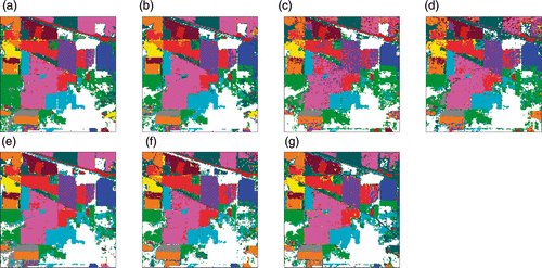
Figure 7. Classification maps of Indian Pines data with SVM classifier using EMAPs of (a) PCA, (b) KPCA, (c) DAFE, (d) DBFE and (e) NWFE, and feature reduction applied on EMAP using (f) NW-NW and (g) KP-NW.

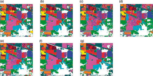
Figure 8. The ground reference data for the Indian Pines image. The segments shown in white boxes are found to be difficult to classify.

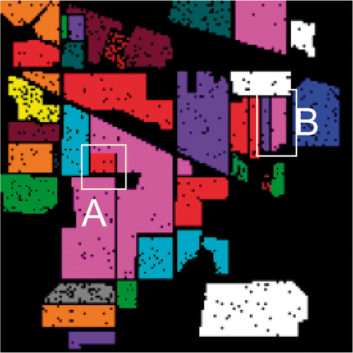
Figure 9. Classification maps for University of Pavia data with RF classifier using (a) Original data (b) PCA, (c) KPCA, (d) DAFE, (e) DBFE and (f) NWFE.

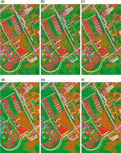
Figure 10. Classification maps for University of Pavia data with SVM classifier using (a) Original data (b) PCA, (c) KPCA, (d) DAFE, (e) DBFE and (f) NWFE.

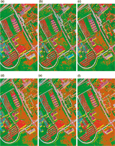
Figure 11. Classification results of University of Pavia data with RF classifier using EMAPS of (a) KPCA, (b) DBFE, (c) NWFE and feature reduction applied on EMAP using (d) DB-DB.

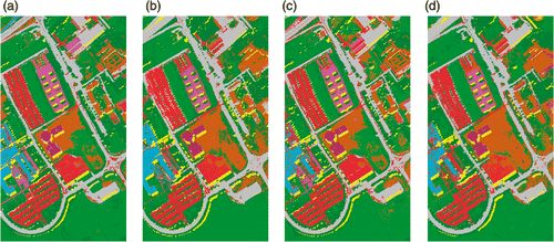
Figure 12. Classification maps of University of Pavia data with SVM classifier using EMAPS of (a) KPCA, (b) DBFE, (c) NWFE and feature reduction applied on EMAP using (d) DB-DB.

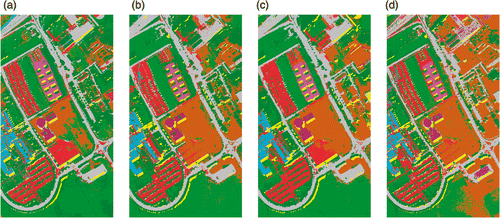
Table 5. Accuracies in percentage for classification of Pavia image with 30 training pixels per class. The best results in terms of accuracy are marked in bold.

Panel A: Results using RF with spectral information only
Class	DBFE	DAFE	NWFE	KPCA
Features	10	8	15	20
1	89.13	90.6	96.54	96.08
2	76.4	74	74.44	72.06
3	88.35	87.82	91.05	82.41
4	67.08	70.94	54.07	50.21
5	100	99.85	99.33	98.88
6	99.68	99.89	99.89	99.26
7	82.07	73.82	83.98	79.85
8	70.84	68.92	57.73	56.5
9	82.12	76.26	79.38	62.58
AA	83.96	82.46	81.82	77.54
OA	77.22	74.89	71	67.25
κ	71.24	68.34	64.13	59.39
Panel B: Results using RF with profiles
Class	DBFEp	DAFEp	NWFEp	KPCAp
Features	150	120	225	300
1	87.63	87.14	98.49	98.79
2	89.12	91.87	94.87	95.52
3	98.64	86.09	99.62	97.66
4	63.17	72.41	69.84	97.42
5	99.85	100	99.92	99.55
6	99.36	99.68	100	99.89
7	87.01	71.89	98.42	98.42
8	87.49	81.58	89.82	87.82
9	90.47	86.95	80.85	62.97
AA	89.20	86.40	92.42	93.12
OA	87.87	84.04	90.77	89.20
κ	84.20	79.39	87.90	85.81
Panel C: Results using SVM with spectral information only
Class	DBFE	DAFE	NWFE	KPCA
Features	10	8	15	20
1	91.12	87.53	89.85	94.81
2	71.27	66.01	63.04	72.39
3	88.87	85.56	89.02	80.60
4	70.84	73.27	64.13	58.50
5	99.70	99.78	99.41	99.03
6	99.79	99.16	99.89	99.47
7	78.68	64.67	72.35	73.28
8	60.13	56.19	54.63	54.08
9	89.60	88.15	88.84	63.77
AA	83.33	80.04	80.13	77.33
OA	72.68	68.52	67.95	66.09
κ	66.32	61.40	60.81	58.15
Panel D: Results using SVM with profiles
Class	DBFEp	DAFEp	NWFEp	KPCAp
Features	150	120	225	300
1	89.72	94.13	96.89	97.94
2	87.66	54.68	81.87	91.11
3	82.26	66.99	95.78	98.72
4	65.46	65.27	68.74	82.61
5	87.06	65.72	99.40	98.95
6	98.52	91.55	98.83	99.57
7	58.01	47.45	82.69	97.71
8	67.83	45.70	63.34	86.54
9	82.76	75.88	91.58	84.37
AA	79.92	67.49	86.57	93.06
OA	75.00	57.53	76.80	89.64
κ	68.43	49.06	71.20	86.56

Table 6. Accuracies in percentage for classification of Pavia image with 100 training pixels per class. The best results in terms of accuracy are marked in bold.

Panel A: Results using RF with spectral information only
Class	DBFE	DAFE	NWFE	KPCA
Features	20	8	18	20
1	91.29	87.70	97.32	97.72
2	80.46	79.37	79.55	70.22
3	84.74	76.69	90.15	87.29
4	63.70	67.17	67.27	58.60
5	100	100	99.93	99.63
6	99.16	99.68	99.89	99.47
7	84.03	76.43	89.27	82.54
8	68.91	63.54	61.26	58.38
9	93.44	88.41	92.15	73.73
AA	85.08	82.11	86.31	80.84
OA	78.37	74.29	75.99	70.03
κ	72.86	67.93	70.33	63.00
Panel B: Results using RF with profiles
Class	DBFEp	DAFEp	NWFEp	KPCAp
Features	300	120	270	300
1	96.21	83.61	99.09	99.37
2	97.01	95.12	95.60	95.06
3	99.84	98.57	100	99.47
4	85.08	69.12	68.79	93.56
5	100	100	99.93	99.77
6	99.89	97.25	100	100
7	98.96	96.60	98.64	99.61
8	98.13	97.24	97.39	91.10
9	81.84	97.89	63.89	61.06
AA	95.22	92.82	91.48	93.2292
OA	95.49	94.71	92.22	90.3661
κ	93.98	92.98	89.56	87.24
Panel C: Results using SVM with spectral information only
Class	DBFE	DAFE	NWFE	KPCA
Features	20	8	18	20
1	92.00	85.77	84.14	97.88
2	76.88	69.54	71.29	68.81
3	85.19	77.37	84.14	88.72
4	67.56	66.51	65.27	69.32
5	99.93	100	99.85	99.70
6	99.16	99.16	98.94	96.73
7	81.29	78.27	81.50	83.24
8	66.19	59.81	57.48	67.56
9	93.24	88.35	94.73	69.78
AA	84.60	80.53	81.93	82.42
OA	76.62	71.13	71.44	73.94
κ	70.88	64.31	64.97	67.30
Panel D: Results using SVM with profiles
Class	DBFEp	DAFEp	NWFEp	KPCAp
Features	300	120	270	300
1	93.14	86.49	98.76	98.98
2	90.71	79.34	84.92	90.95
3	98.57	92.41	94.06	99.24
4	67.98	67.22	76.70	89.23
5	99.85	100	99.63	99.92
6	99.78	94.93	98.42	99.36
7	89.62	81.04	88.24	99.21
8	76.56	71.01	70.45	91.78
9	98.72	97.73	95.63	87.03
AA	90.55	85.57	89.64	95.08
OA	85.18	79.33	81.79	92.78
κ	81.18	74.02	77.16	90.56

Figure 13. A snapshot of University of Pavia region from Google Maps (accessed 02 November 2011). A big part of the image remains unchanged from the date of acquisition of the ROSIS image. The boxes delineates specific areas considered in the discussion to visually compare the geometric stability of the classification results. Imagery ©2011 DigitalGlobe, GeoEye.

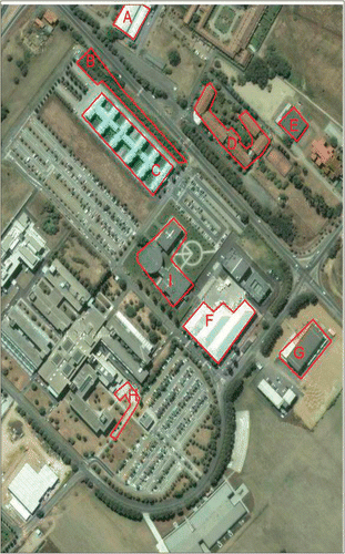
Figure 14. Classification maps of University of Pavia data using 30 training samples per class with RF classifier using (a) KPCA, (b) DAFE, (c) DBFE, (d) NWFE, (e) KPCA _{p ,} (f) DAFE _{p ,} (g) DBFE _p and (h) NWFE _p .

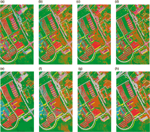
Figure 15. Classification maps of University of Pavia data using 30 training samples per class with SVM classifier (a) KPCA, (b) DAFE, (c) DBFE (d) NWFE, (e) KPCA _{p ,} (f) DAFE _{p ,} (g) DBFE _p and (h) NWFE _p .

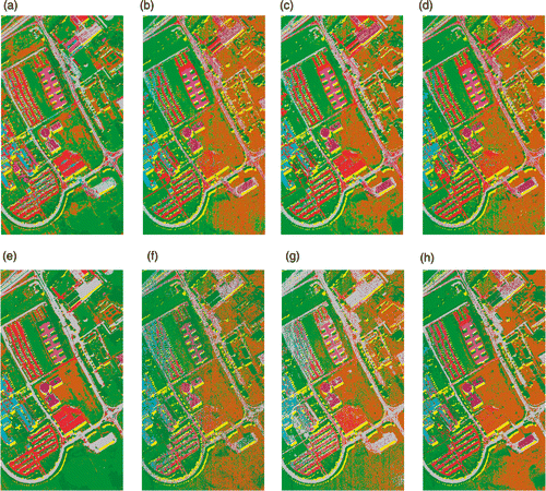
Figure 16. Classification maps of University of Pavia data using 100 training samples per class with RF classifier using (a) KPCA, (b) DAFE, (c) DBFE, (d) NWFE, (e) KPCA _{p ,} (f) DAFE _{p ,} (g) DBFE _p and (h) NWFE _p.

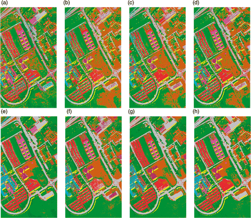
Figure 17. Classification maps of University of Pavia data using 100 training samples per class with SVM classifier using (a) KPCA, (b) DAFE, (c) DBFE, (d) NWFE, (e) KPCA _{p ,} (f) DAFE _{p ,} (g) DBFE _p and (h) NWFE _p .