MMINP: A computational framework of microbe-metabolite interactions-based metabolic profiles predictor based on the O2-PLS algorithm

Figures & data

Figure 1. MMINP workflow. (a) Training MMINP model with pre-processed metabolome (Y: metab(N,M)) and metagenome (X: metag(N,K)) data; N, the sample size of training data; M, the number of metabolites; K, the number of bacteria. step 1) construction of an O2-PLS model with preprocessed microbial genes (X) and metabolites (Y) data; step 2) prediction of metabolites using the model built in step 1; step 3) spearman correlation analysis between measured values and predicted values, metabolites with correlation coefficient greater than 0.4 would be defined as WFMs; step 4) the model will retrain until all the metabolites in the model are WFMs (remove metabolites except WFMs from Y and repeat step 1–3 until all retained metabolites are WFMs). (b) New metagenomes with overlapping genes (overlapping ratio more than ‘minGenesize’) with MMINP model can be predicted by the model. WFMs, well-fitted metabolites.

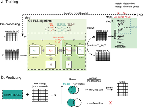
Figure 2. The prediction performance of MMINP. (a) The predicted situation of metabolites. NIM (metabolites not in the model): the input metabolites which are removed during modeling. WPM (well-predicted metabolites): metabolites with a spearman correlation coefficient (predicted versus measured metabolites abundance in testing data) no less than 0.3. PPM (poorly predicted metabolites): metabolites with a spearman correlation coefficient less than 0.3. Assigned: metabolites assigned to putative chemical classes by comparing with the Human Metabolome Database. Unassigned: metabolites without assignment. WFMs (well-fitted metabolites), identical to predicted metabolites (PMs), is the sum of WPMs and PPMs. (b) Barplot of NIMs, PPMs, and WPMs of each putative chemical class. Classes with at least five well-predicted metabolites are displayed. (C) Procrustes analysis on metabolite profiles between predicted and measured values based on Eucildean distance (M² = 0.389, P = 0.001); each line links the predicted and measured features of one sample. Shorter bars (corresponding to a lower M²) indicate that a more similar relationship between the predicted and measured features of the sample. Blue points represent samples from control. Red points represent samples from CD. Yellow points represent samples from UC.

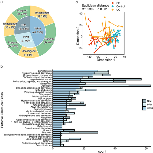
Figure 3. The downstream analysis of MMINP prediction. (a) Comparison of metabolite profiles between CD and Control samples by principal component analysis (PCA) and permutational multivariate analysis of variance based on Euclidean distance matrices using measured (above) and predicted metabolome (below). (b) Boxplot of the median difference of differentially abundant metabolites between CD and control in each putative chemical class. Tested by Wilcoxon rank sum test with Benjamini-Hochberg correction for multiple comparisons (FDR <0.05). Classes with at least five well-predicted metabolites are presented. (c) Over-representation analysis (ORA) on chemical classes associated with the differentially abundant metabolites in each group.

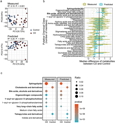
Figure 4. The comparison of prediction performance among O2-PLS, MMINP, MelonnPan, and ENVIM. (a) the bottom part shows the number of PMs and WPMs, while the upper part shows the PM/All ratio, WPM/All ratio, and WPM/PM ratio. All: the input metabolites for modeling. Predicted: metabolites predicted by the model, i.e., metabolites in the model. Wellpredicted: metabolites with a spearman correlation coefficient (predicted versus measured metabolites abundance in testing data) greater than 0.3. (b) Barplot of Precision, Accuracy, Recall and F1 score among O2-PLS, MMINP, MelonnPan, and ENVIM.

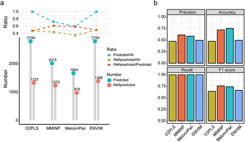
Figure 5. The impact of training sample size on the prediction performance. (a–f) the PM/All ratio (a), WPM/All ratio (b), WPM/PM ratio (c), Precision (d), Accuracy (e), and F1 score (f) of models constructed by training samples with different sizes when predicting metabolites of the test set.

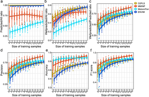
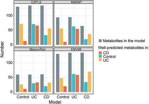
Figure 6. The impact of host disease state on prediction performance. Samples from CD, UC, or control group were respectively used to build the model and apply it to the samples of the other two groups. Barplot shows the number of metabolites. Grey bars represent the number of well-fitted metabolites in each model. Red bars represent the number of well-predicted metabolites using each model to predict samples from CD. Blue bars represent the number of well-predicted metabolites using each model to predict samples from the control. Yellow bars represent the number of well-predicted metabolites using each model to predict samples from UC.

Data availability statement

All the data sets and R scripts used in this manuscript can be downloaded from https://github.com/YuLab-SMU/Supplemental-MMINP.