Ordering taxa in image convolution networks improves microbiome-based machine learning accuracy

Figures & data

Table 1. Different approaches to the microbiome ML limitations discussed in the introduction.

Model	Completing missing data at higher level	Rare elements are taken into account	Smoothing over similar taxa CNN	Smoothing over similar taxa ordering
iMic	V	V	V	V
	Cladogram of averages	Log transform		Dendrogram ordering, such that similar sister taxa are closer in the image
gMic+v	X	V	V	X
		Log transform	GCN
gMic	X	X	V	X
	No use of values	No use of values	GCN
PopPhy-CNN	V	X	V	X
	Cladogram of sums	Relative abundances		No ordering
TopoPhy-CNN	V	X	V	X
	Cladogram of sums	Relative abundances Higher weight for hubs		No ordering
DeepEn-Phy	NN from each lower level to the higher level	X	V, GCN	X
CoDaCoRe	X	V	X	X
		Log transform
TaxoNN	X	X	V	X
			1-dimensional CNN
FCN	X	V	X	X
		If log transform is applied to the input
RF	X	V	X	X
		If log transform is applied to the input
LR	X	V	X	X
		If log transform is applied to the input
SVC	X	V	X	X
		If log transform is applied to the input

Table 2. Table of datasets.

Dataset	Tag	Case	Control	Origin	Species	Reference
IBD	CD or UC	137	120	Stool	70	^Citation46
	CD	94	163
Cirrhosis	Cirrhosis	68	62	Stool	794	^Citation47
Allergy	Milk	74	200	Stool	881	^Citation5
	Nuts	53	221
	Peanut	79	195
CA	Caucasian	96	104	Vagina	151	^Citation48
MF	Male	98	82	Stool	907	^Citation47
Ravel	High Nugent score	97	245	Vagina	530	^Citation48

Figure 1. iMic’s and gMic’s architectures and AUCs.

(a) gMic+v architecture: We position all observed taxa in the leaves of the taxonomy tree (cladogram), and set their value to the preprocessed frequency to each leaf. Each internal node is the average of its direct descendants. These values are the input to a GCN layer with the adjacency matrix of the cladogram. The GCN layer is followed by two fully connected layers with binary output. (b) iMic’s architecture: The values in the cladogram are as in gMic+v. The cladogram is then used to populate a 2-dimensional matrix. Each row in the image represents a taxonomic level. The order in each row is based on a recursive hierarchical clustering of the sample values preserving the structure of the tree. The image is the input of a CNN followed by 2 fully connected layers with binary output. (c) Comparison between model performance: The average AUC is measured on the external test set on nine different phenotypes. Each subplot is a phenotype. The stars represent the significance of the $\mathit{p}$-value (after Benjamini Hochberg correction) on the external test set. If there were differences in the significance on the 10 CVs and the external test set, the different corrected p-value of the 10 CVs is reported in brackets, *-$\mathit{p}\le 0.05$, **-$\mathit{p}\le 0.01$, ***-$\mathit{p}\le 0.001$. For the parallel results of 10 CVs see Supp. Mat. Fig. S2. The rightmost set of plots is the baseline. The green bars are the current best baseline. The light blue bar to the right is the best baseline obtained using the MIPMLP. The central pink bars are the iMic AUC using either a one or two-dimensional CNN. The leftmost bars are for gMic (either gMic or gMic+v). We also added the iMic results to allow for a comparison.

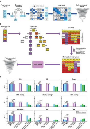
Table 3. Sequential datasets details.

Dataset	Tag	Case	Control	Species	Range # of time steps	Ref
Diabimmune	Milk	53	150
	Peanut	9	194
	Egg	40	163
	All	72	131	87	1–33	^Citation75
DiGiulio case-control study	Preterm	11	29	321	3–158	^Citation76

Table 4. 10 CVs mean performances with standard deviation on external test sets; the std is the std among CV folds.

	iMic-CNN2	iMic-CNN1	gMic +v	gMic	FCN	PopPhy-CNN11	PopPhy-CNN2
IBD	0.961 ± 0.000	0.960 ± 0.000	0.956 ± 0.02	0.958 ± 0.014	0.94 ± 0.00	0.863 ± 0.02	0.834 ± 0.03
CD	0.931 ± 0.006	0.928 ± 0.000	0.936 ± 0.018	0.870 ± 0.023	0.807 ± 0.00	0.716 ± 0.03	0.751 ± 0.016
Ravel	0.946 ± 0.01	0.940 ± 0.000	0.977 ± 0.004	0.959 ± 0.006	0.965 ± 0.01	0.894 ± 0.00	0.898 ± 0.007
Cirrhosis	0.924 ± 0.01	0.896 ± 0.000	0.827 ± 0.013	0.847 ± 0.018	0.832 ± 0.03	0.633 ± 0.01	0.536 ± 0.09
Milk allergy	0.704 ± 0.03	0.704 ± 0.04	0.667 ± 0.104	0.707 ± 0.04	0.710 ± 0.03	0.557 ± 0.04	0.522 ± 0.05
Nut allergy	0.640 ± 0.01	0.659 ± 0.007	0.541 ± 0.081	0.499 ± 0.053	0.513 ± 0.05	0.599 ± 0.08	0.511 ± 0.05
Peanut allergy	0.588 ± 0.03	0.580 ± 0.03	0.535 ± 0.03	0.549 ± 0.073	0.575 ± 0.0	0.539 ± 0.02	0.541 ± 0.05
MF	0.641 ± 0.06	0.645 ± 0.06	0.446 ± 0.04	0.450 ± 0.054	0.51 ± 0.102	0.520 ± 0.06	0.527 ± 0.06
CA	0.681 ± 0.001	0.656 ± 0.01	0.507 ± 0.067	0.544 ± 0.144	0.535 ± 0.07	0.592 ± 0.04	0.610 ± 0.04

Table 5. Features can be added to iMic’s learning. Average AUCs of iMic-CNN2 with and without non-microbial features as well as average results of naive models with non-microbial features. The results are the average AUCs on an external test with 10 CVs $\pm$ their standard deviations (stds).

	iMic-CNN2 + non -microbial	iMic-CNN-only micro	RF+ non-microbial	SVC + non-microbial	LR + non-microbial	FCN + non-microbial
Milk allergy	$0.750\pm 0.04$	$0.704\pm 0.03$	$0.546\pm 0.03$	$0.478\pm 0.04$	$0.600\pm 0.03$	$0.661\pm 0.04$
Nut allergy	$0.680\pm 0.02$	$0.640\pm 0.01$	$0.630\pm 0.03$	$0.661\pm 0.02$	$0.603\pm 0.02$	$0.570\pm 0.03$
Peanut allergy	$0.633\pm 0.04$	$0.588\pm 0.03$	$0.582\pm 0.05$	$0.493\pm 0.05$	$0.427\pm 0.06$	$0.532\pm 0.07$

Figure 2. iMic copes with the ML challenges above better than other methods.

(a) Average test AUC (over 10 CVs) as a function of the different sparsity levels, where the first point is the AUC of the original sparsity level ($72\mathrm{\%}$, “baseline”) on the Cirrhosis dataset. iMic has the highest AUCs for all simulated sparsity levels (purple line). The error bars represent the standard errors. (b) Average change in AUC (AUC – baseline AUC) as a function of the sparsity level on the Cirrhosis dataset. (c) Overall average in AUC change in all the other datasets apart from Cirrhosis. (d) Average AUC as a function of the number of samples in the training set (Cirrhosis dataset). The error bars represent the standard errors of each model over the 10 CVs. (e) Average change in AUC (AUC – baseline AUC) as a function of the percent of samples in the training set. (f) Overall average AUC change over all the algorithms that managed to learn (baseline AUC $>0.55)$ as a function of the percent of samples in the training set. (g) Importance of ordering taxa. The x-axis represents the average AUC over 10 CVs and the y-axis represents the different datasets used. The deep purple bars represent the AUC on the images without taxa reordering, while the light purple bars represent the AUC on the images with the Dendrogram reordering with standard errors. All the differences between the AUCs are significant after Benjamini Hochberg correction $(\mathit{p}$-value $<0.001)$. All the AUCs are calculated on an external test set for each CV. Quite similar results were obtained on the 10 CVs.

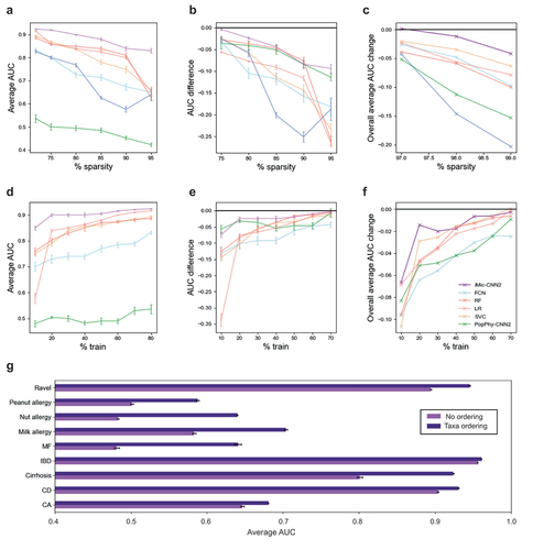
Figure 3. Interpretation of iMic’s results.

(a, b) Cladogram projections: To visualize the taxa contributing to each class, the healthy class (a) and the CD class (b), we projected the most significant microbes back on the cladogram. The purple points on the cladograms represent taxa that are in the top decile of the gradients. The taxa in bold are important taxa that are consistent with the literature. (c, d) Grad-Cam images: Each image represents the average contribution of each input value to the gradients of the neural network back-propagation, as computed by the Grad-Cam algorithm. We put the Grad-Cam after the first CNN layer. The results presented here are from the CD dataset. (c) represents the average gradients for the healthy subjects of the cohort and (d) represents the average gradients for the CD subjects. The color reflects the average values of the gradients, such that the blue colors represent low gradients, and the yellow colors represent the high gradients, using the ‘viridis’ colormap. The differences between the two heatmaps represent the contribution of different taxa to the prediction of different phenotypes. Note that the main contribution to the classification is at the genus and family level (rows 6 and 5). Similar results were obtained for the other datasets (Fig. S11 in Supp. Mat.) (e-h). Interpretation tests on the CD dataset (e), the IBD dataset (f), the Cirrhosis dataset (g), and the Ravel dataset (h). Average AUC values over 10 CVs on the external test set. The x-axis represents the fraction of removed columns. The dark bars represent the performance when all of the columns with Grad-Cams values lower than this fraction have been removed and the light bars represent the performance when the columns with scores above this fraction have been removed. The black line represents the average AUC over 10 CVs of the original model with all the input columns. Results from the other datasets were similar, see Supp. Mat Fig. S11. Removing the top scoring columns always reduced the performance. Removing the bottom scoring columns increases or does not change the AUC.

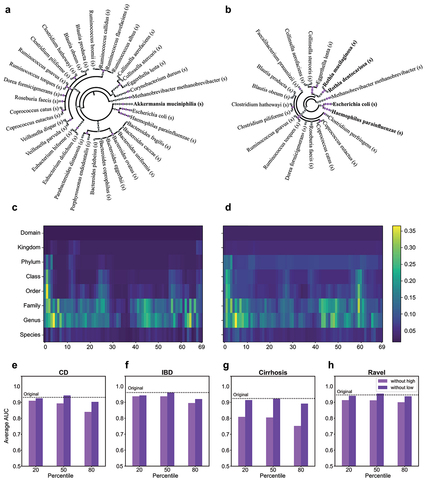
Figure 4. 3D learning.

(a) iMic 3D Architecture: The ASV frequencies of each snapshot are preprocessed and combined into images as in the static iMic. The images from the different time points are combined into a 3D image, which is the input of a 3-dimensional CNN followed by two fully connected layers that return the predicted phenotype. (b) Performance of 3D learning vs PhyLoSTM. The AUCs of the 3D-iMic are consistently higher than the AUCs of the phyLoSTM on all the tags and datasets we checked $(\mathit{n}=5)$. The standard errors among the CVs are also shown. phyLoSTM is the current state-of-the-art for these datasets (two-sided T-test, $\mathit{p}$-value $<0.0005$). To visualize the three-dimensional gradients (as in Figure 3), we studied a CNN with a time window of 3 (i.e., 3 consecutive images combined using convolution). We projected the Grad-Cam images to the R, G, and B channels of an image. Each channel represents another time point where R = earliest, G = middle, and B = latest time point. (c,d) Images after Grad-Cam: Each pixel represents the value of the backpropagated gradients after the CNN layer. The 2-dimensional image is the combination of the three channels above. (i.e., the gradients of the first/second/third time step are in red/green/blue). The left image is for normal birth subjects in the DiGiulio dataset, and the right image is for pre-term birth subjects. (e,f) Grad-Cam projection. Projection of the above heatmaps on the cladogram as in Figure 3. The taxa in bold are important taxa that are consistent with the literature.

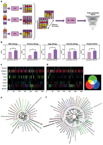
Table 6. Notations.

$\mathit{b}$	ASVs preprocessed vector (only the leaves of the cladogram)
$\mathit{R}$	Raw representation matrix
$\hat{R}$	Rearranged representation matrix
$\mathit{l}$	A taxonomic level (Super-kingdom, Phylum, Class, Order, Family, Genus, Species)
$\mathit{N}$	Number of leaves of the cladogram of means
$C_{\mathit{l},\mathit{i}}$	Hierarchical cluster number $\mathit{i}$ in level $\mathit{l}$
$\mathit{A}$	Adjacency matrix of graph
$\mathit{\sigma }$	Activation function
$\mathit{W}$	Weight matrix in neural network
$\mathit{I}$	Identity matrix
$\mathit{v}$	ASVs frequency vector (all the cladogram’s vertices, and not only the leaves, in contrast with $\mathit{b}$ above)

Table

Algorithm 1: Populating mean cladogram algorithm

1 Input: Cladogram, $\mathit{G}=(\mathit{V},\mathit{E})$, a preprocessed ASVs vector, $\mathit{b}$ 2 Output: A populated cladogram of means, $\mathit{G}$ 3 for $\mathit{l}$ from the maximum cladogram depth to 0 do 4 for each node, $\mathit{v}$, in layer,$\mathit{l}$ do 5 if the layer of $\mathit{v}$ is in $\mathit{b}$ then 6 Assign node $\mathit{v}$ the value from $\mathit{b}$ 7 if $\mathit{v}$ has any children then 8 Assign its children mean to $\mathit{v}$ 9 return $\mathit{G}$

Table

Algorithm 2: Cladogram2matrix algorithm

1 Input: A populated cladogram of means $\mathit{G}=\mathit{V},\mathit{E}$ 2 Output: A matrix $\mathit{R}$ 3 Construct a zero matrix $\mathit{R}$ with the number of rows equal to the layers of the cladogram and the number of columns equal to the number of leaves in the cladogram 4 $\mathit{C}\leftarrow$ Root Node of $\mathit{G}$ 5 for $\mathit{j}$ from 0 to the number of layers of $\mathit{G}$ do 6 $\mathit{i}\leftarrow 0$ 7 $\mathit{Q}\leftarrow \mathit{emptyQueue}$ 8 for each node $\mathit{v}\in \mathit{C}$ do 9 Notice: every node is a sub-tree 10 if node does not have any children then 11 $\mathit{R}(\mathit{i},\mathit{j})\leftarrow$ abundance of node $\mathit{v}$ 12 else 13 for $\mathit{k}$ from 1 to number of leaves of node $\mathit{v}$ do 14 $\mathit{R}(\mathit{i},\mathit{j})\leftarrow$ abundance of node $\mathit{v}$ 15 $\mathit{i}\leftarrow \mathit{i}+1$ 16 Push children of node v into queue $\mathit{Q}$ 17 $\mathit{i}\leftarrow \mathit{i}+1$ 18 $\mathit{C}\leftarrow \mathit{Q}$ 19 return R

Table

Algorithm 3: Reordering algorithm, REA

1 Input: $\mathit{R}\in {\mathbb{R}}^{8\times \mathit{N}}$, $\mathit{l}$ level of taxonomy 2 Output: $\hat{R}$, rearranged matrix $\mathit{R}$ 3 $\hat{R}$ $\leftarrow \mathit{\varphi }$ 4 Annotate: R in level l: $b_1,b_2,\dots ,b_N$ 5 $C_{\mathit{l},1},\dots ,C_{\mathit{l},\mathit{k}}$ $\leftarrow \mathit{Dendrogram}(b_1,b_2,\dots ,b_N)$ 6 Temp $\leftarrow \mathit{\varphi }$ 7 for Cluster in $C_{\mathit{l},1},\dots ,C_{\mathit{l},\mathit{k}}$ do 8 for taxa in Cluster do 9 Append taxa column to Temp if $\mathit{l}<8$ then 10 Temp $\leftarrow \mathit{REA}(\mathit{Temp},\mathit{l}+1)$ 11 Append Temp to $\hat{R}$ 12 return $\hat{R}$

van der Giessen J, Binyamin D, Belogolovski A, Frishman S, Tenenbaum-Gavish K, Hadar E, Louzoun Y, Petrus Peppelenbosch M, van der Woude CJ, Koren O, et al. Modulation of cytokine patterns and microbiome during pregnancy in IBD. Gut. 2020;69(3):473–486. doi:10.1136/gutjnl-2019-318263.

 PubMed Web of Science ®Google Scholar

Human Microbiome Project Consortium. Structure, function and diversity of the healthy human microbiome. Nature. 2012;486(7402):207. doi:10.1038/nature11234.

 PubMed Web of Science ®Google Scholar

Goldberg MR, Mor H, Magid Neriya D, Magzal F, Muller E, Appel MY, Nachshon L, Borenstein E, Tamir S, Louzoun Y, et al. Microbial signature in IgE-mediated food allergies. Genome Med. 2020;12(1):1–18. doi:10.1186/s13073-020-00789-4.

 Web of Science ®Google Scholar

Ravel J, Gajer P, Zaid Abdo GMS, Koenig SSK, McCulle SL, Karlebach S, Gorle R, Russell J, Tacket CO, Brotman RM. Vaginal microbiome of reproductive-age women. Proc Natl Acad Sci USA. 2011;108(supplement_1):4680–4687. doi:10.1073/pnas.1002611107.

 PubMed Web of Science ®Google Scholar

Vatanen T, Kostic AD, d’Hennezel E, Siljander H, Franzosa EA, Yassour M, Kolde R, Vlamakis H, Arthur TD, Hämäläinen A-M, et al. Variation in microbiome LPS immunogenicity contributes to autoimmunity in humans. Cell. 2016;165(4):842–853. doi:10.1016/j.cell.2016.04.007.

 PubMed Web of Science ®Google Scholar

DiGiulio DB, Callahan BJ, McMurdie PJ, Costello EK, Lyell DJ, Robaczewska A, Sun CL, Goltsman DSA, Wong RJ, Shaw G, et al. Temporal and spatial variation of the human microbiota during pregnancy. Proc Natl Acad Sci USA. 2015;112(35):11060–11065. doi:10.1073/pnas.1502875112.

 PubMed Web of Science ®Google Scholar

Data availability statement

All datasets are available at https://github.com/oshritshtossel/iMic/tree/master/Raw_data.