Figures & data
Table 1. Behavioral ethogram used in this study.
Figure 1. Changes in fecal microbial diversity over time. Figures 1a-b represent changes in Shannon index (alpha diversity) at the bacterial genera and species levels over time (mean ±95% confidence interval). Figures 1c-h represent changes in beta diversity (bray-curtis dissimilarity) at the bacterial genera level (c-e) and species level (f-h) over time. Bacterial genera and species were classified based on 16S rRNA sequencing and shotgun metagenomic sequencing, respectively. * signifies that the Shannon indices of the two groups were significantly different at that time-point (t-test, p < .05). p-values in figures 1c-h represent the results of PERMANOVA (100 permutations) at the particular phase of the experiment.
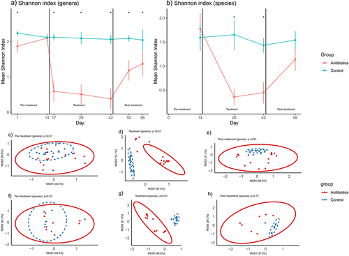
Figure 2. Relative abundances of a) bacterial genera and b) bacterial species in feces. Bacterial genera and species were classified based on 16S rRNA sequencing and shotgun metagenomic sequencing, respectively.
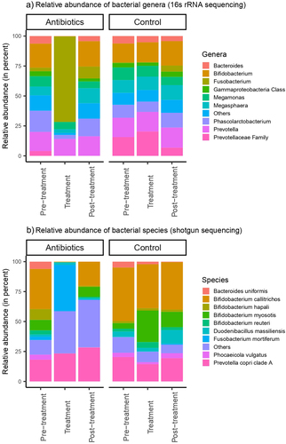
Figure 3. Differentially abundant fecal bacterial genera (a-c) and species (d-f) across different phases of the experiment based on LefSe analysis. Bacterial genera and species were classified based on 16S rRNA sequencing and shotgun metagenomic sequencing, respectively.
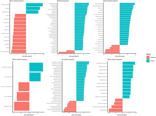
Figure 4. Within-group changes in behaviors (a-e) of the common marmosets during the course of the experiment. Bar-plots represent mean ± standard error. p-values highlighted were estimated from mixed effects general linear models built at the group level. *- p-value <.05, **- p-value <.01, ***- p-value <.001. Piloerection and genital display did not change significantly in zero-inflated negative binomial regression models.
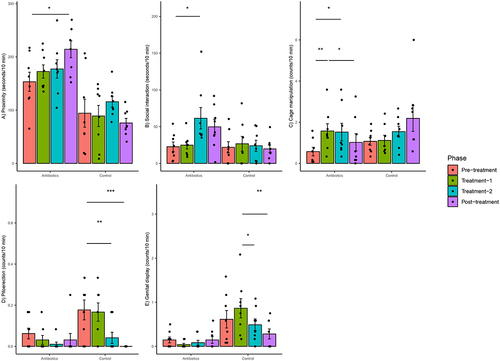
Figure 5. Differentially abundant predicted functional pathways across different phases of the experiment based on LefSe analysis. Only those pathways that were correlated with behaviors (p <.05) are displayed here.
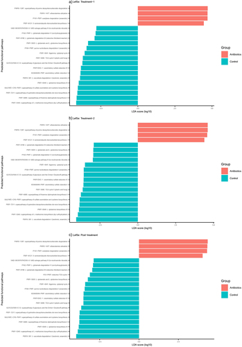
Figure 6. Changes in fecal metabolite and metabolic pathways abundances across time (based on untargeted metabolomics). Figures 5A-C represent principal component analysis plots of the untargeted metabolomic runs for a) pre-treatment phase, b) treatment phase and c) post-treatment phase. Figures 5D-E represent differentially enriched metabolic pathways (top 25) during treatment and post-treatment phases. Metabolic pathways were significantly enriched (p-values after false discovery rate correction < 0.05).
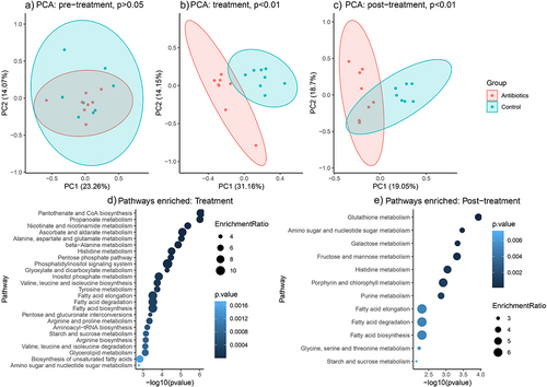
Figure 7. Within-group changes in select fecal metabolites and neurotransmitters (A-K) during the course of the experiment. The y-axes represent normalized abundances of these compounds derived from untargeted GC-MS. Bar-plots represent mean ± standard error. p-values highlighted were estimated from mixed effects general linear models built at the group level. *- p-value <.05, **- p-value <.01, ***- p-value <.001.
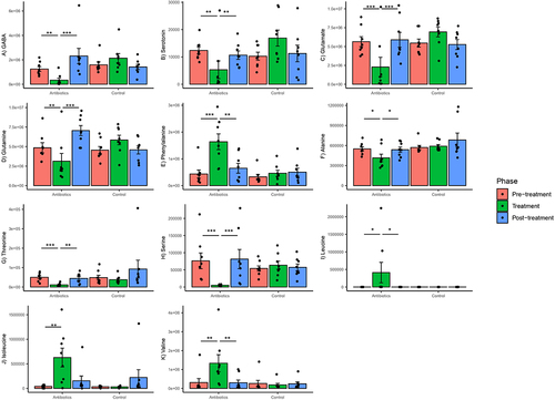
Figure 8. Within-group changes in fecal bile acids concentrations (A-N) during the course of the experiment. Bar-plots represent mean ± standard error. p-values highlighted were estimated from mixed effects general linear models built at the group level. *- p-value <.05, **- p-value <.01, ***- p-value <.001. “BA”- bile acids, “P:S ratio”- Primary:secondary bile acids ratio.
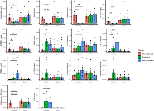
Figure 9. Within-group changes in fecal short-chain fatty acids concentrations (a-e) during the course of the experiment. Bar-plots represent mean ± standard error. p-values highlighted were estimated from mixed effects general linear models built at the group level. *- p-value <.05, **- p-value <.01, ***- p-value <.001.
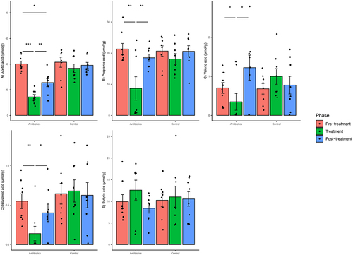
Figure 10. Within-group changes in the urinary cortisol concentrations: a) during the course of experiment and b) before and after exposure to a stressor. Bar-plots represent mean ± standard error. p-values highlighted were estimated from mixed effects general linear models built at the group level. *- p-value <.05, **- p-value <.01, ***- p-value <.001.
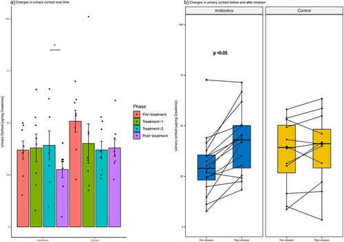
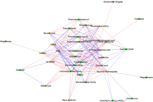
Figure 11. Networks of correlations between fecal metabolites and observed behavior. Red and blue edges represent negative and positive correlations, respectively. Nodes in orange and green represent fecal metabolites and genera based on 16S rRNA sequencing, respectively. Significant correlations (p-values after false discovery rate correction < .01) are presented here.