Numerical and experimental hydrodynamic study of a coolant distributor for grinding applications

Figures & data

Figure 1. (a) 2D view of the distributor geometry; (b) different elements of the grinding process.

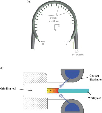
Figure 2. Experimental setup of the distributor hydraulic loop.

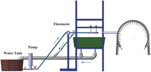
Figure 3. (a) Experimental and PIV setup; (b) test section.

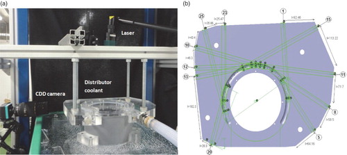
Table 1. Parameters for PIV acquisition.

Parameters	Adaptation
Method of correlation	Intercorrelation
Laser	Wave length = 532 nm
Particles	Hollow glass spheres: diameter = 10 μm; density = 1.1 g/cm^3; refractive index = 1.52
Dimension of ZI and pixels	64 × 64 pixels; 1 pixel = 0.019 mm
	Lint = 64 × 0.019 mm
Number of images	n = 100
Time between two laser pulsations Δt	Δt = 30, 40 and 70 μs
Recovery	50%
Time between two image pairs	0.067 s

Figure 4. Refined tetrahedral mesh in the wall region.

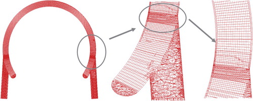
Table 2. Geometrical parameters.

Parameters	Values
Outlet diameters	d = 0.8, 2.5 and 4.2 mm
Number of outlets	n = 25, 26 and 27

Figure 5. Computed hydrodynamic fields: (a) velocity contours; (b) pressure contours in the axial cross-section y = 1.

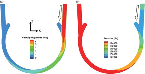
Figure 6. Sections along the distributor.

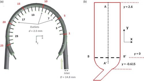
Figure 7. Computed velocity field (m.s⁻¹) for nozzle diameters of (a) d = 0.8 mm, (b) d = 2.5 mm and (c) d = 4.2 mm in the streamwise cross-section of Nozzle 5.

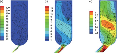
Figure 8. Numerical velocity magnitude along the distributor (axis AA′) for nozzle diameters (a) d = 0.8 mm, (b) d = 2.5 mm and (c) d = 4.2 mm for Q = 3.8 m³/h.

Figure 9. Numerical velocity magnitude along the distributor (axis BB′) for nozzle diameters (a) d = 0.8 mm, (b) d = 2.5 mm and (c) d = 4.2 mm for Q = 3.8 m³/h.

Figure 10. Computed and theoretical velocity magnitudes at the centerline for different nozzle diameters for Q = 3.8 m³/h.

Figure 11. Computed hydrodynamic fields for the axial cross section y = 1 for: (a) TKE contours (m²/s²); (b) TKE dissipation rate contour.

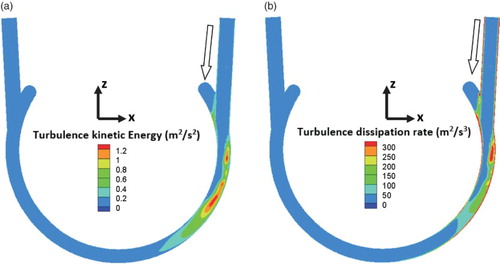
Figure 12. Computed normalized TKE at the centerline for different nozzle diameters for Q = 3.8 m³/h.

Table 3. Internal relative pressure for different nozzle diameters and inlet flow rates.

	Theoretical pressure (Pa)		Numerical pressure (Pa)		Experimental pressure (Pa)
Q (m^3/h)	3.8	6	3.8	6	3.8	6
d = 0.8 mm	3.53 × 10^6	8.79 × 10^6	4.30 × 10^6	10.80 × 10^6	-	-
d = 2.5 mm	3.70 × 10^4	9.22 × 10^4	3.83 × 10^4	9.32 × 10^4	2.35 × 10^4	7.9 × 10^4
d = 4.2 mm	4.60 × 10^3	1.16 × 10^4	2.60 × 10^3	-	-	-

Figure 13. Comparison between PIV experimental results and CFD simulations of the velocity field in a cross-section for Q = 3.8 m³/h and d = 2.5 mm.

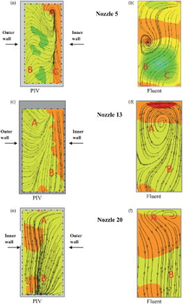
Figure 14. CFD compared to theoretical pressure profiles along the distributor for different nozzle diameters for Q = 3.8 m³/h.

Figure 15. CFD compared to theoretical and experimental pressure profiles along the distributor for nozzle diameter d = 2.5 mm and Q = 3.8 m³/h.

Figure 16. CFD computed and theoretical distributed flow rates at outlets for different nozzle diameters, Q = 3.8 m³/h.

Figure 17. CFD compared to theoretical and experimental distributed flow rates at outlets for nozzle diameter d = 2.5 mm and Q = 3.8 m³/h.

Figure 18. (a) Distributor pressure as a function of nozzle diameter; (b) Flow-rate–pressure relationship for the distributor.

Table 4. Computed jet Reynolds number for different nozzle diameters and inlet flow rates.

	Rej		H/d
Q(m^3/h)	3.8	6
d = 0.8 mm	68,720	108,632	7.5
d = 2.5 mm	22,175	35,075	2.4
d = 4.2 mm	13,440	–	1.4