CFD simulations of flow and dust dispersion in a realistic urban area

Figures & data

Figure 1. Top view of the residential community located in Hangzhou city. The dashed red line (y = 100 m, z = 1.6 m) represents the line to abstract data for comparisons.

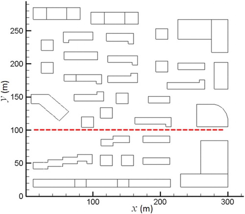
Figure 2. (a) Computational domain and horizontal grid, (b) grid distribution in the vertical direction, and (c) comparison of velocity distribution along the dashed line marked in Figure 1 between the basic grid, coarser grid and finer grid cases.

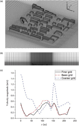
Figure 3. Vertical inflow profiles of the mean velocity, turbulent kinetic energy and dissipation rate.

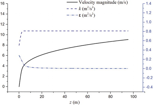
Table 1. Sampled dust aerosol size distribution during the dust storm of the year 2000.

Diameter range (μm)	<0.4	<0.7	<1.1	<2.1	<3.3	<4.7	<5.8	<9.0
Concentration (μg·m^−3)	73.62	89.82	163.44	340.12	590.41	914.32	1208.78	1621.03
Content (%)	3.49	4.26	7.75	16.14	28.02	43.39	57.37	76.94

Figure 4. Staggered obstacle array in the experiment and simulation for (a) the computational domain and (b) the grid settings.

Figure 5. Comparisons of mean streamwise velocity between the experimental data and the present simulation for (a) lateral profiles at the z = H/2 horizontal plane and (b) vertical profiles at the y = 0 vertical plane.

Note: □ = data measured with a pulsed-wire anemometer; △ = data measured with a hot-wire anemometer; red solid line = the present numerical results.

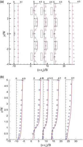
Figure 6. The wind velocity distribution in the 1.6 m horizontal plane above the ground under the due-north wind condition case with a 10 m/s reference height wind velocity.

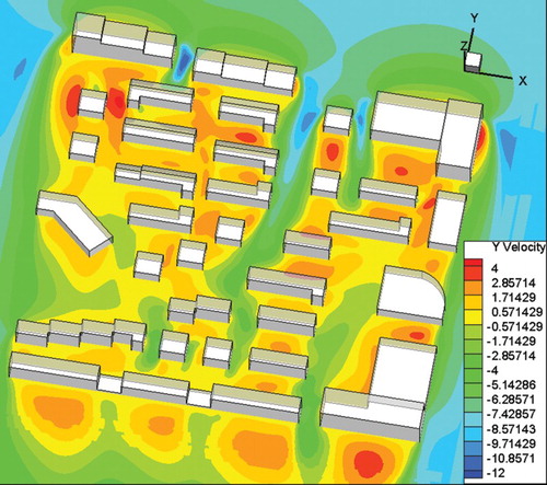
Figure 7. Distribution of dust concentration under the due-north wind condition for (a) the wind velocity vector and (b) the 1.6 m horizontal plane above the ground.

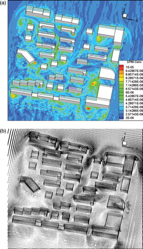
Figure 8. Distribution of the dust concentration in several vertical planes parallel to the primary wind direction under the due-north wind condition for (a) x = 40 m, (b) x = 90 m, (c) x = 180 m, and (d) x = 240 m.

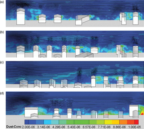
Figure 9. Iso-surfaces of dust concentration under the due-north wind condition with values of (a) 4.2e−6 kg/m³ and (b) 6.3e−6 kg/m³.

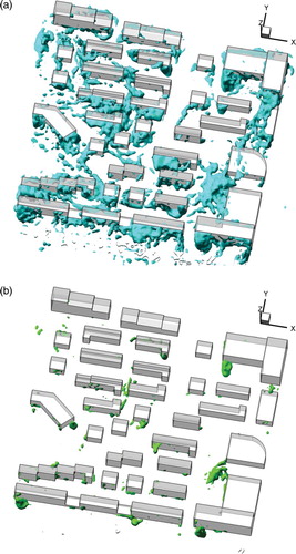
Figure 10. Distribution of the y-component wind velocity under the northwest wind condition for (a) the wind velocity vector, (b) the dust concentration, and (c) the 1.6 m horizontal plane above the ground.

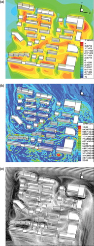
Figure 11. Distribution of the y-component wind velocity under the northeast wind condition for (a) the wind velocity vector, (b) the dust concentration, and (c) the 1.6 m horizontal plane above the ground.

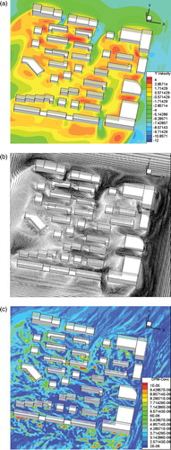
Figure 12. Distributions of dust concentration in the 1.6 m horizontal plane above the ground under the due-north wind condition and with particle-wall impact restitution coefficient sets of: (a) normal 0.25, tangential 0.25, (b) normal 0.50, tangential 0.50, (c) normal 0.75, tangential 0.75, and (d) normal 0.50, tangential 0.7.

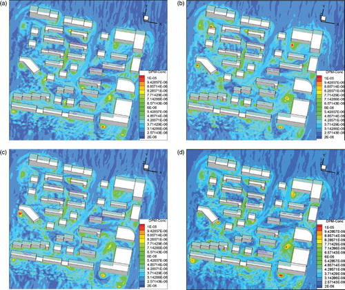
Figure 13. Distribution of dust concentration in the 1.6 m horizontal plane above the ground under the northwest wind condition for (a) the reflect wall condition and (b) the capture wall condition.

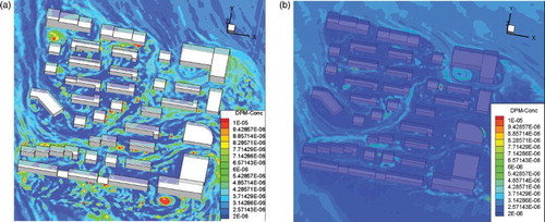
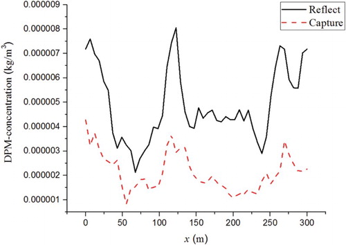
Figure 14. Spatial variation of particle concentration along the dashed line marked in Figure 1 under the reflection wall condition and the capture wall condition.