Analysis of the aerodynamic impact of the dispenser stance for the separation of cluster munitions

Figures & data

Table 1. Computational parameters.

M	907.18 kg
Ixx	27.12 kg m^2
Iyy	488.09 kg m^2
Izz	488.09 kg m^2
Forward ejector location	1.23 m aft of store nose
Aft ejector location	1.75 m aft of store nose
Center of gravity	1.42 m aft of store nose

Figure 1. Pressure contours in the initial position.

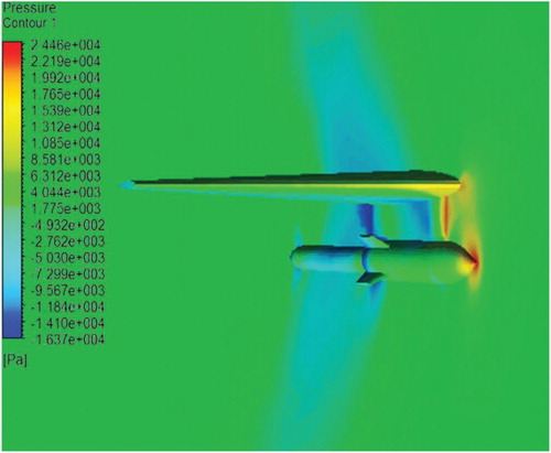
Figure 2. Separation trajectory of the store.

Figure 3. Comparison of the center of gravity over time for the simulated and experimental results.

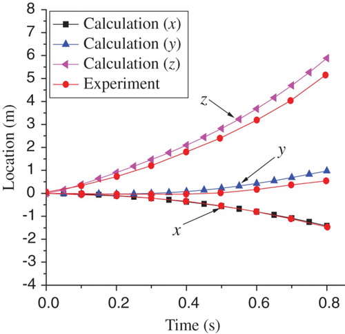
Figure 4. Comparison of the angular orientation over time for the simulated and experimental results.

Figure 5. Model of cluster munitions.

Figure 6. Computational model of the submunition.

Figure 7. Local mesh for the submunition.

Figure 8. Volume mesh for the calculation area.

Table 2. Computational conditions.

Mach number	3
Mass of the submunition	27 kg
Free stream temperature	300 K
Free stream pressure	101325 Pa
Initial separation angle	3°, 5°, 7°
Initial separation velocity	8 m/s, 16 m/s

Figure 9. Photograph of the experimental model.

Figure 10. Schlieren photograph of the experimental model in position 1, for Ma = 3 and y₁ = l/d_c = 0.8333, for (a) α = 3°, (b) α = 5°, and (c) α = 7°.

Figure 11. Schlieren photograph of the experimental model in position 2, for Ma = 3 and y₂ = l/d_c = 1.5201, for (a) α = 3°, (b) α = 5°, and (c) α = 7°.

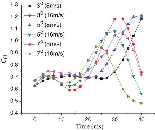
Figure 12. Comparison of the drag coefficient for the simulated and experimental results under different conditions.

Note: Ma = 3; y₁ = l/d_c = 0.8333 for position 1, y₂ = l/dc = 1.5201 for position 2.

Figure 13. Comparison of the lift coefficient for the simulated and experimental results under different conditions.

Note: Ma = 3; y₁ = l/dc = 0.8333 for position 1, y₂ = l/dc = 1.5201 for position 2.

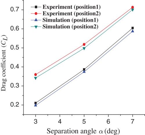
Figure 14. Comparison of the pitching moment coefficient for the simulated and experimental results under different conditions.

Note: Ma = 3; y₁ = l/dc = 0.8333 for position 1, y₂ = l/dc = 1.5201 for position 2.

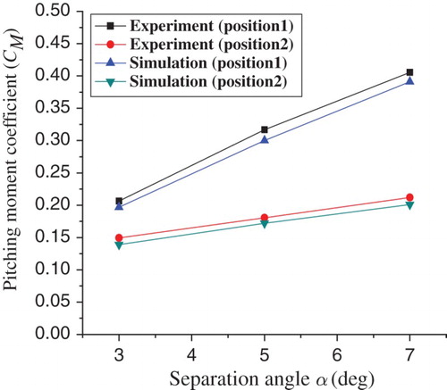
Figure 15. Pressure contours of the separation for α = 3° and v₀ = 8 m/s at (a) t = 0 ms, (b) t = 10 ms, (c) t = 30 ms, and (d) t = 40 ms.

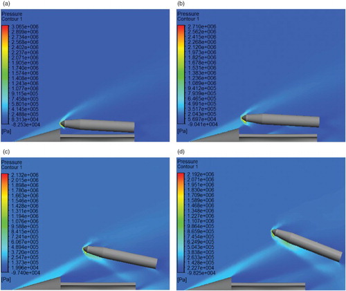
Figure 16. Pressure contours of the separation for α = 7° and v₀ = 16 m/s at (a) t = 0 ms, (b) t = 10 ms, (c) t = 30 ms, and (d) t = 40 ms.

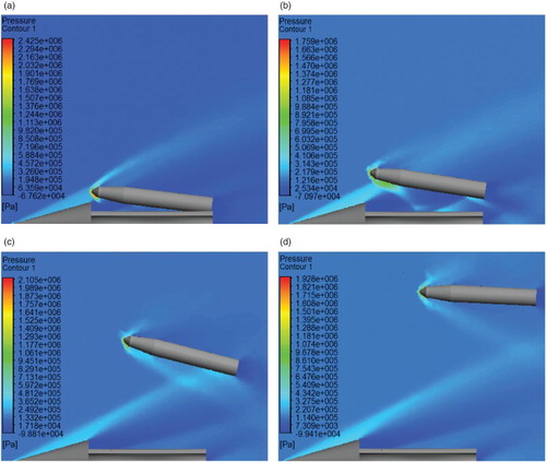
Figure 17. The process of mesh reconstruction for α = 7° and v₀ = 16 m/s at (a) t = 0 ms, (b) t = 10 ms, (c) t = 20 ms, and (d) t = 30 ms.

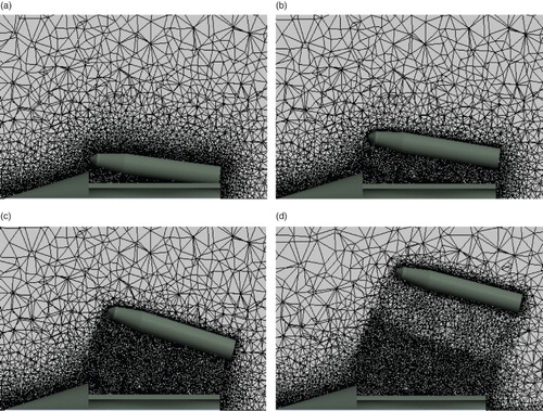
Figure 18. The surface pressure contours of the submunition for α = 3° and v₀ = 8 m/s at (a) t = 0 ms, (b) t = 10 ms, (c) t = 20 ms, and (d) t = 30 ms.

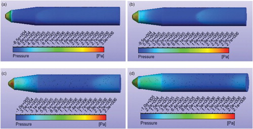
Figure 19. The surface pressure contours of the submunition for α = 7° and v₀ = 16 m/s at (a) t = 0 ms, (b) t = 10 ms, (c) t = 20 ms, and (d) t = 30 ms.

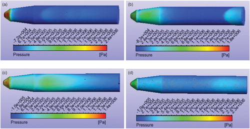
Figure 20. Separation trajectories for (a) α = 3° and v₀ = 8 m/s, (b) α = 5° and v₀ = 8 m/s, (c) α = 7° and v₀ = 8 m/s, (d) α = 3° and v₀ = 16 m/s, (e) α = 5° and v₀ = 16 m/s, and (f) α = 7° and v₀ = 16 m/s.

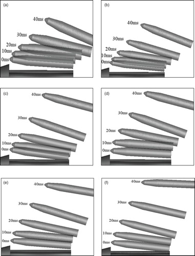
Figure 21. Relative velocity in the x direction for the six conditions.

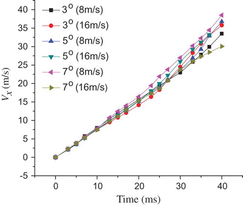
Figure 22. Relative velocity in the y direction for the six conditions.

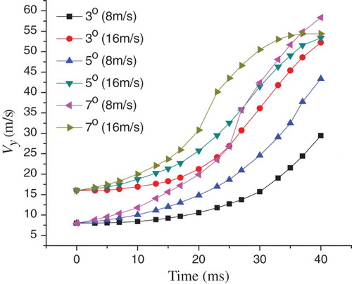
Figure 23. Center of gravity displacement for the six conditions.

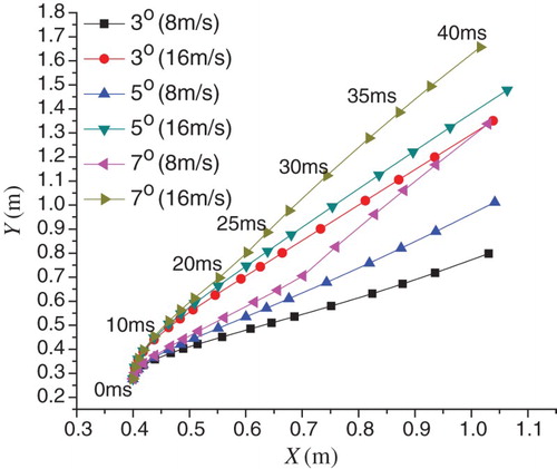
Figure 24. Angular velocity with time for the six conditions.

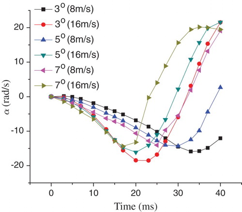
Figure 25. Lift coefficients for the six conditions.

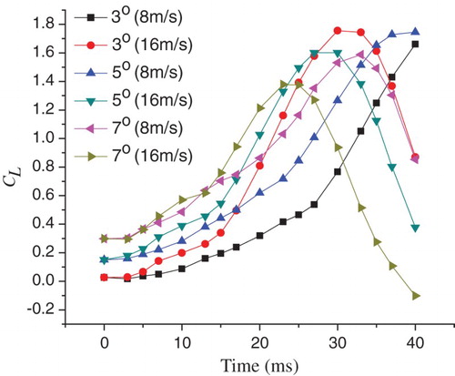
Figure 26. Drag coefficients for the six conditions.