Viscous numerical wave tank for Bragg resonance by cnoidal and Stokes waves

Figures & data

Figure 1. A sketch of the adaptive mesh refinement.

Figure 2. Schematic diagram of the viscous numerical wave tank.

Figure 3. A criterion of different wave theories.

Figure 4. Water surface elevations by a damping zone at various time instants in an empty tank.

Figure 5. Arrangement of the numerical setup and computational domain.

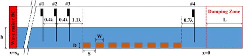
Table 1. Comparisons of the grid level by different types of refinement.

	Water	Free surface	Damping zone	Air
Min/max
levels	and	and		and
Uniform grid
Semi-uniform grid
Dynamic grid adaptation

Figure 6. A comparison of (a) reflections and (b) transmissions of Bragg scattering by water waves over a series of submerged rectangular breakwaters.

Figure 7. Comparisons of velocity profiles of Stokes Bragg resonance (a) before 1st breakwater at and (b) before 1st breakwater at .

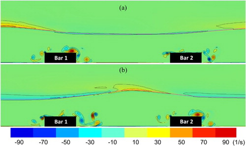
Figure 8. Numerical results of (a) vorticity fields, (b) velocity vector fields and (c) adaptive grids at phase for the Stokes Bragg resonance.

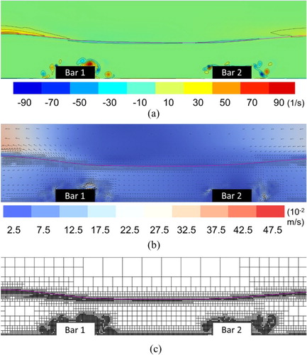
Figure 9. Numerical results of (a) vorticity fields, (b) velocity vector fields and (c) adaptive grids at phase for the Stokes Bragg resonance.

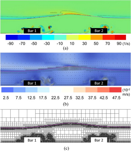
Figure 10. A time history distributions ( sec) of particles trajectories at different positions for the Stokes Bragg resonance.

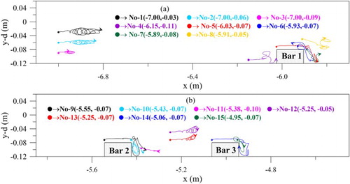
Figure 11. Numerical results of (a) vorticity fields and (b) velocity vector fields at phase for the Stokes Bragg resonance of oil.

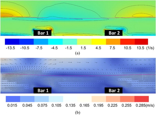
Figure 12. Numerical results of (a) vorticity fields and (b) velocity vector fields at phase for the Stokes Bragg resonance of oil.

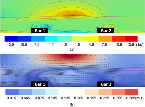
Figure 13. Comparisons of velocity profiles between Stokes waves and cnoidal waves under Bragg resonance condition (a) before 1st breakwater and (b) on the top center of 1st breakwater.

Figure 14. Numerical results of (a) vorticity fields, (b) velocity vector fields and (c) adaptive grids at phase for the cnoidal Bragg resonance.

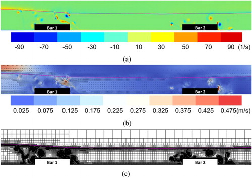
Figure 15. Numerical results of (a) vorticity fields, (b) velocity vector fields and (c) adaptive grids at phase for the cnoidal Bragg resonance.

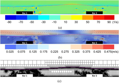
Figure 16. A time history distributions ( sec) of particles trajectories at different positions for the cnoidal Bragg resonance.

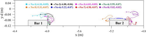
Table 2. Comparisons of scattering parameters for Stokes and cnoidal Bragg resonances.

Stokes resonance	0.7072	0.5859	15.66%	20.81	29431
cnoidal resonance	0.5956	0.5454	34.78%	83.23	57143

Figure 17. A comparison of (a) uniform and (b) semi-uniform grids at phase for the Stokes Bragg resonance.

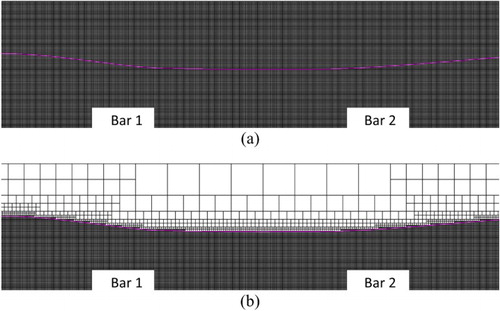
Figure 18. A comparison of (a) uniform and (b) semi-uniform grids at phase for the Stokes Bragg resonance.

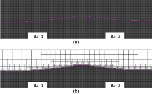
Figure 19. A vorticity contour obtained by a simulation of semi-uniform grid at phases (a) and (b) for the Stokes Bragg resonance.

Table 3. Comparisons of grid cost by different type of refinement (physical time: 20 s).

Type of the refined mesh	Number of cells	Computing time (hours)	Speed up	Interval of Time step	Total time step
Uniform grid			–^a	1.31∼1.63 ()
Semi–uniform grid		59.1	^a	0.94∼3.61 ()
			–^b
Dynamic grid adaption		9.82	^a	0.56∼7.23 ()
			^b

^awith respect to uniform grid.

^bwith respect to semi-uniform grid.