Figures & data
Table 1. Climatic parameters recorded at the Lahijan (Rasht) stations over the time period covered in this study.
Figure 1. Location of the study area and meteorological stations from which the measurement data were obtained.
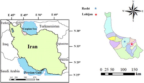
Figure 2. Schematic structure of the SVR and SVR-FA models used for evaporation prediction.
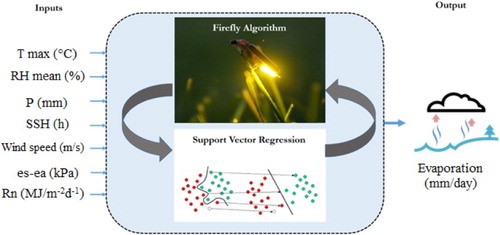
Figure 3. Relation between precipitation and evaporation for the selected time period in this study (days): (a) Lahijan and (b) Rasht.
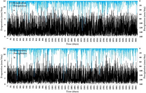
Table 2. Various scenarios considered as inputs of the models.
Table 3. Pearson correlation coefficient values between the main meteorological parameters measured at the Lahijan station.
Figure 4. Measured evaporation amounts versus evaporation values predicted by SVR (black circles) and SVR-FA (blue circles) for different scenarios in Lahijan station and 1:1 line (dash line).
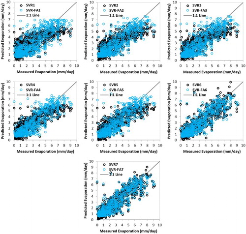
Figure 5. Measured evaporation amounts versus evaporation values predicted by SVR (black circles) and SVR-FA (blue circles) for different scenarios in Rasht station and 1:1 line (dash line).
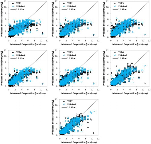
Table 4. Pearson correlation coefficient values between the main meteorological parameters measured at the Rasht station.
Table 5. SVR and SVR-FA RMSE and correlation coefficient values in the training (testing) phases for the seven scenarios.
Table 6. SVR and SVR-FA RMSE values and number of underpredicted or overpredicted days (n) in the testing phases for the seven scenarios at the Lahijan (Rasht) stations.
Figure 6. RMSE values of SVR and SVR-FA models with different scenarios related to measured evaporation amounts higher and lower than average in Lahijan (circle) and Rasht (triangle) stations.
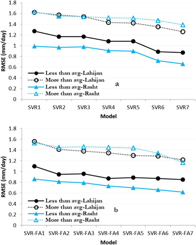
Figure 7. RMSE values (mm/day) for predicting evaporation in Lahijan station (two top figures) and Rasht station (two bottom figures) by SVR and SVR-FA models for 2-mm intervals of evaporation.
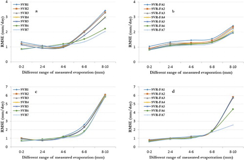
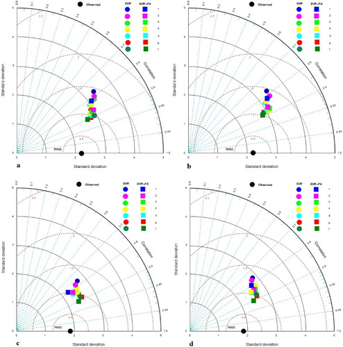
Figure 8. Statistical indices including standard deviation, correlation coefficient and RMSE in the form of Taylor diagram for SVR and SVR-FA models in Lahijan (training Phase)(a), Lahijan (testing Phase)(b), Rasht (training phase)(c) and Rasht (testing phase)(d).