Thin and sharp edges bodies-fluid interaction simulation using cut-cell immersed boundary method

Figures & data

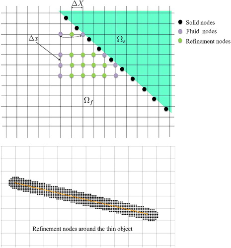
Figure 1. Illustration of the Eulerian and Lagrangian meshes, where $\mathrm{\Omega }s$ and $\mathrm{\Omega }f$ denote the solid region and fluid region, respectively. The velocity interpolation coefficients from the locally refined mesh at the fluid-solid interface are also shown. The velocities at the new nodes are interpolated from the old nodes within the square region.

Table

1. Solve the N-S equations for the entire computational domain using projection method.

2. Compute ${\mathit{d}}_{\mathit{x}}$ and ${\mathit{d}}_{\mathit{y}}$ for the small rectangular region around the thin object with respect to the degree of refinement $dx=DX,DY/2^N$, $d{t}_{new}=DT/2^N$ where $N=1,2,\dots ,n$.

3. Interpolate ${\mathit{u}}_1$ and ${\mathit{v}}_1$ for the boundaries of the rectangular region around the thin object.

4. Compute the boundaries of the refined mesh node around the thin object.

5. Determine the volume fraction for the solid in the local cells and compute the velocity.

6. Compute the momentum exchange.

7. Compute ${\mathit{u}}_{\mathit{d}}$ and ${\mathit{v}}_{\mathit{d}}$ for the volume fraction based on the solid digitizer.

8. Compute the intermediate velocity and pressure

9. Compute ${\mathit{d}}_{\mathit{x}}$ and ${\mathit{d}}_{\mathit{y}}$ and update the values accordingly.

10. Compute the coordinates $\left(x_{pr}\text{and}{y}_{pr}\right)$ for the moving particles using the Crank–Nicholson method.

11. Correct the velocity and pressure.

For elastic structure

12. Compute the (FEM) for solid equations to calculate the space displacement for every time step under the forces from the fluid at Equation (21) after 2-stage correction.

13. Return to Step 1.

Figure 2. Illustration of the background mesh and locally refined mesh within vicinity of the thin object.

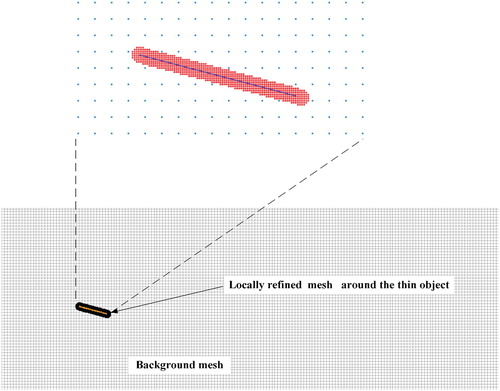
Table 1. Flow around stationary circular cylinder: $C_D$, $C_L$ and St at $R_e=100$.

Source	Drag coefficient, $C_D$	Lift coefficient, $C_L$	Strouhal number, $St$
AMR-IBM	3.255	0.9913	0.2997
(Schäfer & Turek, 1996)	3.22–3.24	0.990–1.010	0.295–0.305
(Verkaik et al., 2014)	3.2258	0.98934	0.30061
(Lee & Lee, 2012)	3.33	1.03	0.299
CFD software	3.227	0.9723	0.2985

Figure 3. Time-histories of Lift and Drag coefficient AMR-IBM algorithm vs CFD at Re = 100.

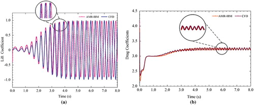
Figure 4. The regression analysis for (a) Drag coefficient and (b) lift coefficient factor using AMR-IBM and CFD simulation.

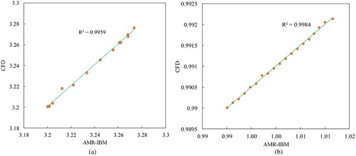
Figure 5. Drag coefficient curves for different $\mathrm{\Delta }x$.

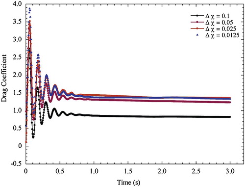
Figure 6. Variations of the (a) lift coefficient and (b) drag coefficient with time for flow around a stationary rigid thin object at $R_e=200$ obtained using the AMR-IBM algorithm. The lift and drag coefficients obtained from the IBM algorithm with full mesh refinement are plotted for comparison.

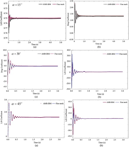
Figure 7. Velocity contour for flow around a stationary rigid thin object (a) AMR-IBM algorithm, (b) Fine mesh.

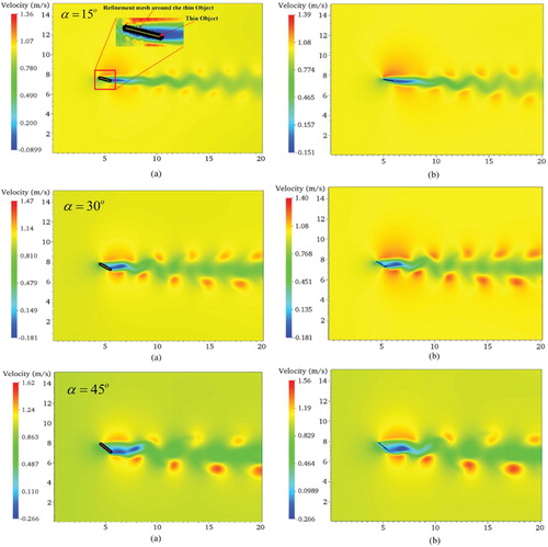
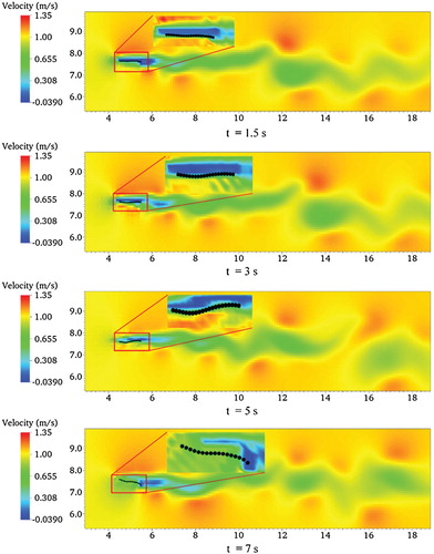
Figure 8. Velocity contour of the moving thin object inclined at an angle of attack 45° at (a) t = 1.5 s, (b) t = 3.5 s, and (c) t = 8.0 s obtained using the AMR-IBM algorithm.

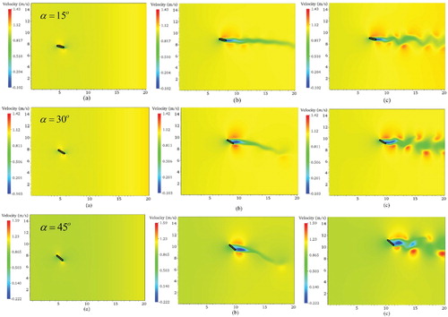
Figure 9. The domain and boundary conditions for the flexible filament 2D problem.

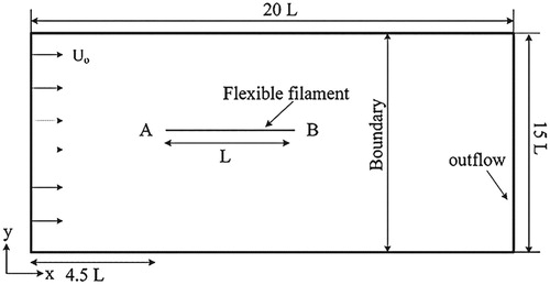
Figure 10. Snapshots of the deformed flexible filament at different time steps. Note that a fixed mesh was used for the fluid flow whereas an adaptive mesh is used within proximity of the thin elastic structure to capture the physics of fluid-solid interaction.

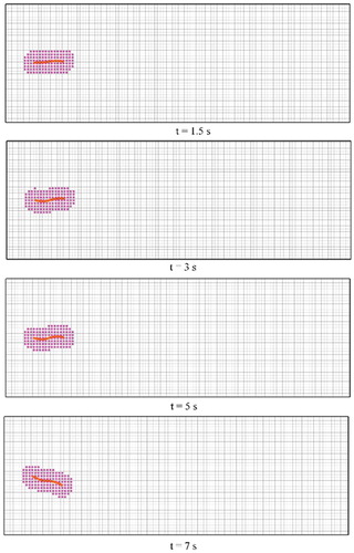
Figure 11. Flapping motion of a single filament immersed in fluid.

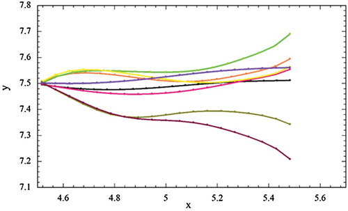
Figure 12. Two-dimensional flexible filament on velocity and geometry deformation distribution at different time step.

Schäfer, M., & Turek, S. (1996). Benchmark computations of laminar flow around a cylinder. In Flow Simulation with High-Performance Computers II, Volume 52 of Notes on Numerical Fluid Mechanics, Vieweg, 52 (pp. 547–566). doi: 10.1007/978-3-322-89849-4_39

 Google Scholar

Verkaik, A. C., Hulsen, M. A., Bogaerds, A. C. B., & van de Vosse, F. N. (2014). An overlapping domain technique coupling spectral and finite elements for fluid flow. Computers & Fluids, 100, 336–346. doi: 10.1016/j.compfluid.2014.05.026

 Web of Science ®Google Scholar

Lee, J., & Lee, S. (2012). Fluid–structure interaction analysis on a flexible plate normal to a free stream at low Reynolds numbers. Journal of Fluids and Structures, 29, 18–34. doi: 10.1016/j.jfluidstructs.2011.12.012

 Web of Science ®Google Scholar