Large eddy simulations of wind loads on an external floating-roof tank

Figures & data

Table 1. SGS models used widely in LES.

SGS model	Equations
SM	${\nu }_{SGS}\text{ = }\rho {L_s}^2\sqrt{2{\overline{S}}_{ij}{\overline{S}}_{ij}}$; $L_s=min\left(\kappa d,C_s\mathrm{\Delta }\right)$
DSM	$({\nu }_{SGS}{)}_f=\left(C_D{{\mathrm{\Delta }}_1}^2\sqrt{2{\overline{S}}_{ij}{\overline{S}}_{ij}}\right)$; $({\nu }_{SGS}{)}_g=\left(C_D{{\mathrm{\Delta }}_2}^2\sqrt{2{\hat{S}}_{ij}{\hat{S}}_{ij}}\right)$; $L_{ij}=(\tau {}_{ij}{)}_{fg}-[{\left({\tau }_{ij}\right)}_f{]}_g$; $L_{ij}+\frac{1}{3}{L}_{kk}{\delta }_{ij}=C_D{M}_{ij}$; $M_{ij}=2\left[{{\mathrm{\Delta }}_2}^2\sqrt{2{\hat{S}}_{ij}{\hat{S}}_{ij}}{\hat{S}}_{ij}-{{\mathrm{\Delta }}_1}^2\stackrel{ˆ}{\sqrt{2{\overline{S}}_{ij}{\overline{S}}_{ij}}{\overline{S}}_{ij}}\right]$; $C_D=\frac{⟨M_{ij}{L}_{ij}⟩}{⟨M_{ij}{M}_{ij}⟩}$
WALE	${\nu }_{SGS}=\rho {L_s}^2\frac{{\left({S_{ij}}^d{S_{ij}}^d\right)}^{3/2}}{{\left({\overline{S}}_{ij}{\overline{S}}_{ij}\right)}^{5/2}+{\left({S_{ij}}^d{S_{ij}}^d\right)}^{5/4}}$; $L_s=min\left(kd,C_w{V}^{1/3}\right)$ ; ${S_{ij}}^d=\frac{1}{2}\left({{\overline{g}}_{ij}}^2+{{\overline{g}}_{ji}}^2\right)-\frac{1}{3}{\delta }_{ij}{{\overline{g}}_{kk}}^2$; ${\overline{g}}_{ij}=\frac{\mathrm{\partial }{\overline{u}}_i}{\mathrm{\partial }{x}_j}$
WMLES	${\nu }_{SGS}=min\left[{\left(\kappa d_w\right)}^2,{\left(C_{S_{mag}}\mathrm{\Delta }\right)}^2\right]\sqrt{2{\overline{S}}_{ij}{\overline{S}}_{ij}}\left\{1-\exp \left[-{\left(\frac{y^{+}}{25}\right)}^3\right]\right\}$; $\mathrm{\Delta }=min\left[max\left(C_w{d}_w,C_w{h}_{max},h_{wn}\right),h_{max}\right]$

Figure 1. A computational model for the turbulent flow around the flat roof and open-topped tank models (Macdonald et al., 1988).

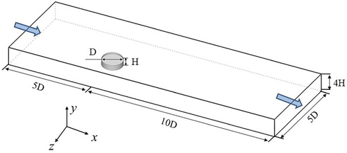
Figure 2. Computational meshes for the benchmark tank models (Macdonald et al., 1988): (a) flat roof tank, (b) open-topped tank.

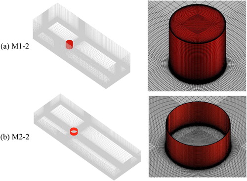
Table 2. A summary of the grid-independence test parameters.

Case	Number of grid nodes	H/D	b/D	SGS model	y/H	Re	y^+
M1-1	434,816	1	0.025	DSM	57%	2.9×10^5	0∼3.5
M1-2	1078,266	1	0.025	DSM	57%	2.9×10^5	0∼1.3
M1-3	1585,436	1	0.025	DSM	57%	2.9×10^5	0∼0.7
M1-4	1393,796	1	0.025	DSM	57%	2.9×10^5	0∼1.2
M2-1	1436,532	0.5	0.025	DSM	62%	2.5×10^5	0∼1.0
M2-2	2046,492	0.5	0.025	DSM	62%	2.5×10^5	0∼0.9
M2-3	4363,652	0.5	0.025	DSM	62%	2.5×10^5	0∼0.7
M2-4	4441,072	0.5	0.025	DSM	62%	2.5×10^5	0∼1.0

Figure 3. Time-averaged pressure coefficients on the two tanks using different meshes: (a) flat roof tank, (b) open-topped tank.

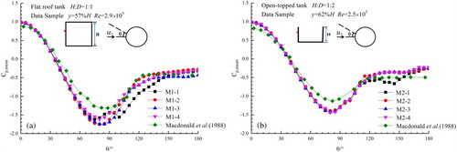
Figure 4. Time-averaged pressure coefficients on the two tanks from different SGS models: (a) flat-roof tank, (b) open-topped tank.

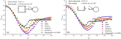
Figure 5. Root-mean-square of the wind pressure coefficients on the two tanks from different SGS models: (a) flat-roof tank, (b) open-topped tank.

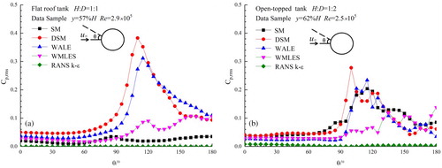
Figure 6. Instantaneous vorticity fields around two tanks at t = 5 computed from LES and RANS: (a) flat-roof tank, (b) open-topped tank.

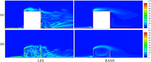
Figure 7. A schematic of the external floating-roof tank model at the maximum liquid level.

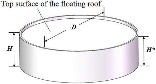
Table 3. A summary of the computations conducting for the external floating-roof tank.

				Re
Model	h/H*	Grid nodes	SGS	Case1	Case2	Case3	Case4
TANK 1	25%	2,101,168	DSM	5.47×10^5	1.09×10^6	1.64×10^6	2.19×10^6
TANK 2	50%	1,089,488	DSM	5.47×10^5	1.09×10^6	1.64×10^6	2.19×10^6
TANK 3	75%	1,058,368	DSM	5.47×10^5	1.09×10^6	1.64×10^6	2.19×10^6
TANK 4	100%	1,076,264	DSM	5.47×10^5	1.09×10^6	1.64×10^6	2.19×10^6

Figure 8. Time-averaged pressure coefficients on the external wall of the tank at different Reynolds numbers: (a) h = 25%H*, (b) h = 50%H*, (c) h = 75%H*, (d) h = 100%H*.

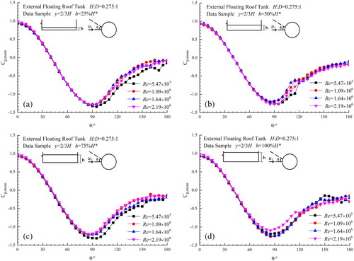
Figure 9. Time-averaged pressure coefficients on the internal wall of the tank at different Reynolds numbers: (a) h = 25%H*, (b) h = 50%H*, (c) h = 75%H*, (d) h = 100%H*.

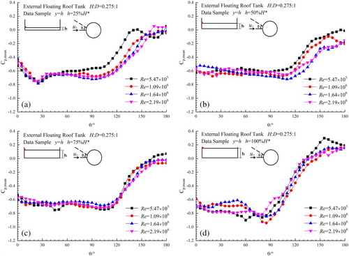
Figure 10. Instantaneous vorticity fields and streamlines at t = 5 around the external floating-roof tank at h = 25%H* and different Reynolds numbers: (a) Re = 5.47×10⁵, (b) Re = 1.09×10⁶, (c) Re = 1.64×10⁶, (d) Re = 2.19×10⁶.

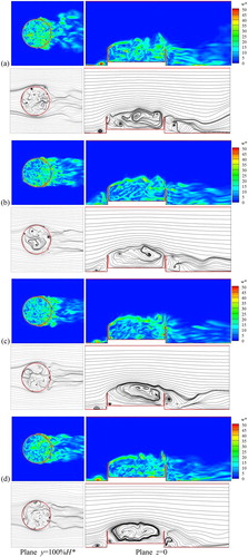
Figure 11. Instantaneous vorticity fields and streamlines at t = 5 around the external floating-roof tank at h = 100%H* and different Reynolds numbers: (a) Re = 5.47×10⁵, (b) Re = 1.09×10⁶, (c) Re = 1.64×10⁶, (d) Re = 2.19×10⁶.

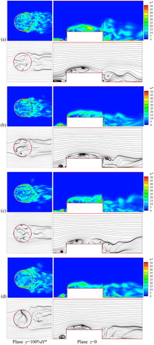
Figure 12. Time-averaged pressure coefficients on the external wall of the tank at different liquid levels: (a) Re = 5.47×10⁵, (b) Re = 2.19×10⁶.

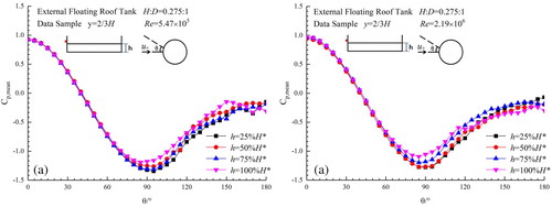
Figure 13. Time-averaged pressure coefficients on the internal wall of the tank at different liquid levels: (a) Re = 5.47×10⁵, (b) Re = 2.19×10⁶.

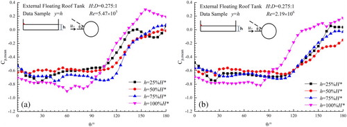
Figure 14. Instantaneous wall pressure coefficients of the tank at h = 25%H* and Re = 2.19×10⁶: (a) external wall, (b) internal wall.

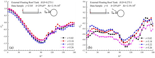
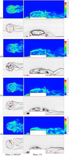
Figure 15. Instantaneous vorticity fields and streamlines at t = 5 around the external floating-roof tank at Re = 5.47×10⁵ and different liquid levels: (a) h = 25%H*, (b) h = 50%H*, (c) h = 75%H*, (d) h = 100%H*.

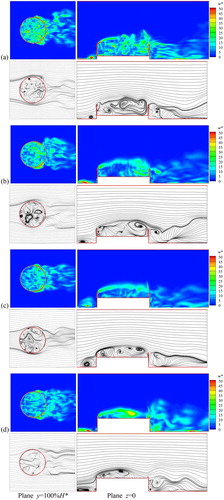
Figure 16. Instantaneous vorticity fields and streamlines at t = 5 around the external floating-roof tank at Re = 2.19×10⁶ and different liquid levels: (a) h = 25%H*, (b) h = 50%H*, (c) h = 75%H*, (d) h = 100%H*.

Macdonald, P. A., Kwok, K. C. S., & Holmes, J. D. (1988). Wind loads on circular storage bins, silos and tanks: Point pressure measurements on isolated structures. Journal of Wind Engineering and Industrial Aerodynamics, 31, 165–188. doi: 10.1016/0167-6105(88)90003-7

 Web of Science ®Google Scholar