A numerical study for the assessment of air pollutant dispersion with chemical reactions from a thermal power plant

Figures & data

Figure 1. Ekibastuz SDPP-1, Kazakhstan.

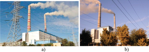
Figure 2. Parameters of the calculated area.

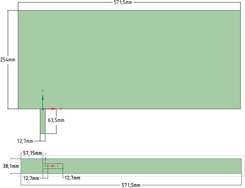
Figure 3. The computational domain grid.

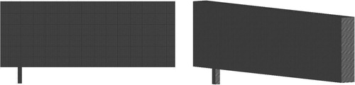
Figure 4. Boundary conditions of the reactor (OXY plane).

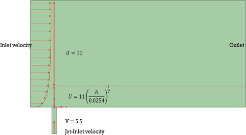
Figure 5. Boundary conditions of the reactor (OYZ plane).

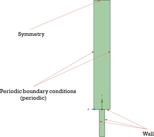
Figure 6. Comparison of the profile of U-velocity for various transverse sections.

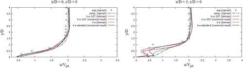
Figure 7. Comparison of the profile of V-velocity for various transverse sections.

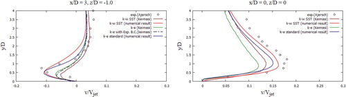
Figure 8. Comparison of the profile of W-velocity for various transverse sections.

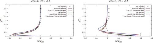
Figure 9. Map of the calculated area.

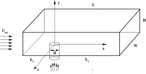
Figure 10 Computational grid of the computational domain.

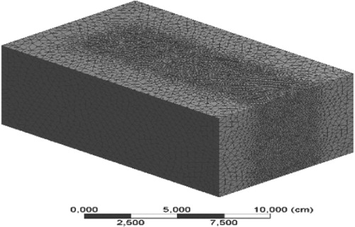
Figure 11. (a) horizontal section and (b) vertical section in the central plane, z/D = 0.

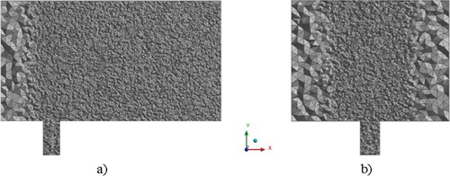
Figure 12. Boundary conditions of the reactor (OYZ plane).

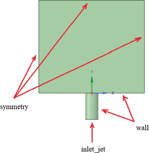
Figure 13. Mean flow rates in the central plane, z/D = 0: (Crabb et al., 1981) (o), Majander & Siikonen (2006) (-) LES (-).

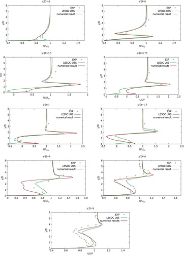
Figure 14. The mean proportion of the mixture in the central plane, z/D = 0: (Crabb et al., 1981) (o), Majander & Siikonen (2006) (-) LES (-).

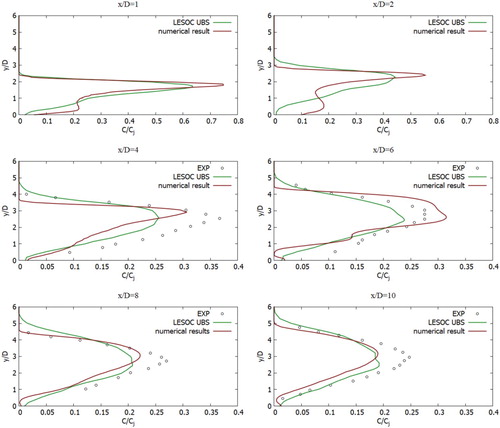
Figure 15. Scheme of the calculated area.

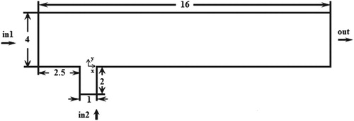
Figure 16. Numbering the outer boundaries of the solution domain.

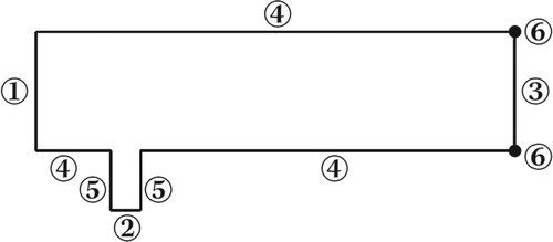
Table 1. Sequence of variables and equations at the boundaries of the $◯1$–$◯6$ domain.

Var.	$◯1$	$◯2$	$◯3$	$◯4$	$◯5$	$◯6$
u	$u_{wind}(1-e^{-5\zeta })$	u = 0	${\displaystyle \frac{\mathrm{\partial }u}{\mathrm{\partial }x}}=0$	u = 0	u = 0	u = 0
W	w = 0	Equation (1)	${\displaystyle \frac{\mathrm{\partial }w}{\mathrm{\partial }x}}=0$	w = 0	w = 0	w = 0
P	Equation (2)	p = $p_{atm}$	Equation (2)	Equation (2)	Equation (2)	Equation (2)
$Y_A$	$Y_A=0$	$Y_A=0$	${\displaystyle \frac{\mathrm{\partial }{Y}_A}{\mathrm{\partial }x}}=0$	${\displaystyle \frac{\mathrm{\partial }{Y}_A}{\mathrm{\partial }y}}=0$	${\displaystyle \frac{\mathrm{\partial }{Y}_A}{\mathrm{\partial }x}}=0$	${\displaystyle \frac{\mathrm{\partial }{Y}_A}{\mathrm{\partial }y}}=0$
$Y_B$	$Y_B=1$	$Y_B=1$	${\displaystyle \frac{\mathrm{\partial }{Y}_B}{\mathrm{\partial }x}}=0$	${\displaystyle \frac{\mathrm{\partial }{Y}_B}{\mathrm{\partial }y}}=0$	${\displaystyle \frac{\mathrm{\partial }{Y}_B}{\mathrm{\partial }x}}=0$	${\displaystyle \frac{\mathrm{\partial }{Y}_B}{\mathrm{\partial }y}}=0$

Figure 17. Calculate computational grid.

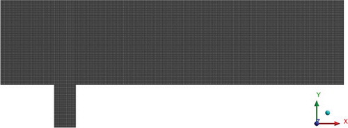
Figure 18. The velocity streamlines comparison: the upper result is the calculations of Schonauer and Adolph (2005), the lower result is the obtained results in this work.

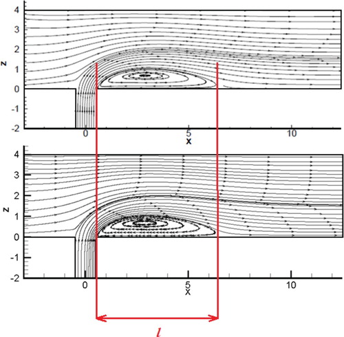
Figure 19. Comparative velocity contour analysis: left plots – results from Schonauer and Adolph (2005), the right-hand plots are the values obtained in the course of this work: (a) horizontal speed u (b) vertical speed v.

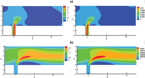
Figure 20. Comparative analysis of the results of the substance distribution: the left graphs – the values of Schonauer and Adolph (2005), the right-hand plots are the obtained results in this work: (a) concentration of substance A, (b) concentration of substance B, (c) concentration of substance C.

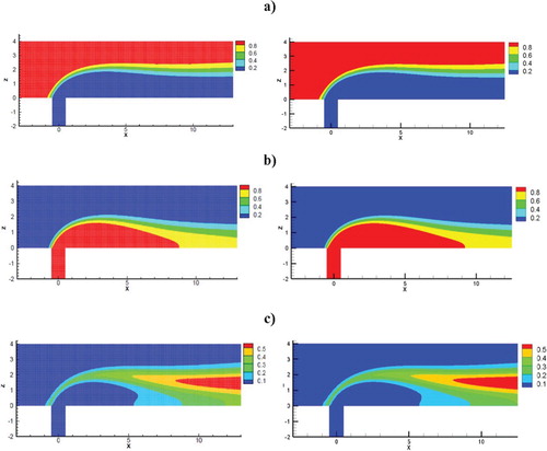
Figure 21. Configuration of computing area for thermal power plant.

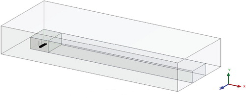
Figure 22. Parameters and dimensions of the calculated area.

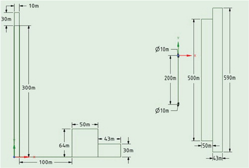
Table 2. Parmameters of species.

	Parameters
Species	Density (kg/m^3)	Viscosity (w/m-K)	Cp (Specific Heat) (j/kg-K)	Thermal Conductivity (w/m-K)	Molecular Weight (kg/kmol)	Standard State Entropy (j/kgmol-K)
O2	1.2999	1.919 × 10^−5	piecewise-polynomial	0.0246	31.9988	205026.9
NO	1	1.72 × 10^−5	piecewise-polynomial	0.0454	30.0061	210640
NO2	1	1.72 × 10^−5	piecewise-polynomial	0.0454	46.0055	239909.6
H2O	0.5542	1.34 × 10^−5	piecewise-polynomial	0.0261	18.01534	188696.4
HNO3	1504	0.011	piecewise-polynomial	0.0454	63.01287	266389.2
Air	1.225	1.7894 × 10^−5	1006.43	0.0242	28.966	194336
CO	1.1233	1.75 × 10^−5	piecewise-polynomial	0.025	28.01055	197531.6
CO2	1.7878	1.37 × 10^−5	piecewise-polynomial	0.0145	44.00995	213720.2

Figure 23. (a) computational grid and (b) bottom view of the grid.

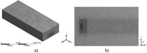
Figure 24. (a) section along the axis OXY and (b) section along the axis OYZ.

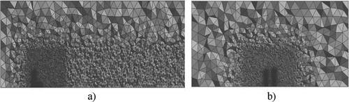
Figure 25. View of the chimneys and buildings.

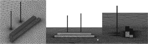
Table 3. Parmameters of geometry.

Geometry parameters (m)	First chimney coordinates (300 m)	Second chimney coordinates (330 m)
X = 10,000	X = 1000	X = 1000
Y = 1800	Y = 0	Y = 0
Z = 4000	Z = 2100	Z = 1900

Figure 26. Boundary conditions of the computational domain.

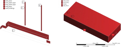
Figure 27. Visualization of the spread of concentrations: (a-d) CO and CO₂, (e-h) NO and NO₂, (i-l) NO₂ and HNO₃.

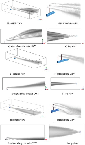
Figure 28. Comparison of profiles of the CO, CO₂ mass fractions in points: x = 1500, 2000, 2500, 3000, 10,000 and z = 2000.

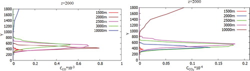
Figure 29. Comparison of profiles of the NO, NO₂ of mass fractions in points: 1500, 2000, 2500, 3000, 10,000 and z = 2000.

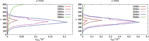
Figure 30. Comparison of profiles of the H₂O, NO₂, HNO₃ mass fraction in points: 1500, 2000, 2500, 3000, 10,000 and z = 2000.

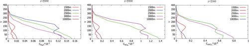
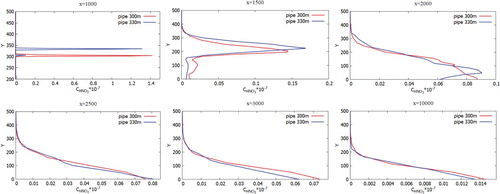
Figure 31. Comparison of profiles of the CO mass fraction at specified points for two various heights of chimneys (300.0 and 330.0 m).

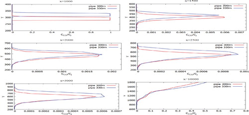
Figure 32. Comparison of profiles of the NO mass fraction at specified points for two various heights of chimneys (300.0 and 330.0 m).

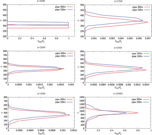
Figure 33. Comparison of profiles of the H₂O mass fraction at the specified points for two various heights of chimneys (300.0 and 330.0 m).

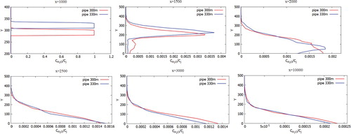
Figure 34. Comparison of profiles of the CO₂ mass fraction at specified points for two various heights of chimneys (300.0 and 330.0 m).

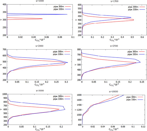
Figure 35. Comparison of profiles of the NO₂ mass fraction at specified points for two various heights of chimneys (300.0 and 330.0 m).

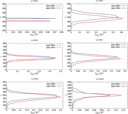
Figure 36. Comparison of profiles of the NO₂ mass fraction at the specified points for two various heights of chimneys (300.0 and 330.0 m).

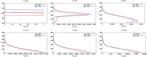
Figure 37. Comparison of profiles of the HNO₃ mass fraction at the specified points for two various heights of chimneys (300.0 and 330.0 m).

Crabb, D., Durao, D., & Whitelaw, J. (1981). A round jet normal to a crossflow. Transactions of the ASME: Journal of Fluids Engineering, 103(1), 568–580. https://doi.org/10.1115/1.3240764

 Web of Science ®Google Scholar

Majander, P., & Siikonen, T. (2006). Large-eddy simulation of a round jet in a cross-flow. International Journal of Heat and Fluid Flow, 27(3), 402–415. https://doi.org/10.1016/j.ijheatfluidflow.2006.01.004

 Web of Science ®Google Scholar

Schonauer, W., & Adolph, T. (2005). FDEM: The evolution and application of the finite difference element method (FDEM) program package for the solution of partial differential equations, Abschlussbericht des Verbundprojekts FDEM, Universitä Karlsruhe. http://www.rz.uni-karlsruhe.de/rz/docs/FDEM/Literatur/fdem.pdf.

 Google Scholar