Improved method for identifying Manning’s roughness coefficients in plain looped river network area

Figures & data

Figure 1. Location of the study area and the spatial distribution of rivers, pumps, sluices, and gauging stations. The main water conservancy projects at the boundary of the CGPA are marked in red. Gauging stations are of two types: B1 to B8 and H1 to H12. The water-level time series data measured by these two types of stations are used for providing boundary conditions for the model simulations and for calibrating the Manning’s roughness coefficients by minimizing the overall discrepancies between the simulated and the measured data, respectively.

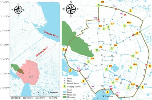
Table 1. Summary of dataset series and sources.

Dataset type	Application	Dataset resolution	Source
Cross-sectional data	Model development	One survey section at 100-m intervals	Changshu Water Bureau
Water conservancy project data	Model development	Location and properties of each project	Changshu Water Bureau
Water-level time series data	Model calibration	Automatically measured every 15 min	Water gauging stations during experiment from Changshu Water Bureau
Water conservancy project operation data	Model calibration	Automatically recorded during each operation	Real-time system during experiment from Changshu Water Bureau

Table 2. Summary of parameter settings in optimization model and statistics of simulation model.

Optimization model		Simulation model
Particle population	20	Number of pumping stations	59
Number of generations	400	Number of sluice structures	71
${\omega }_{min};{\omega }_{max}$	0.4; 0.9	Number of river-reaches	313
${\text{C}}_1$; ${\text{C}}_2$	2; 2	Number of cross-sections	1060
$v_{min}$; $v_{max}$	−0.002; 0.002	Length of simulated river network (km)	138
$p_{min}(n_{min})$; $p_{max}(n_{max})$	0.025; 0.045	Boundaries	8

Figure 2. 1D dynamic model structure of the river networks in the study area as built using InfoWorks ICM software.

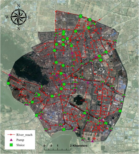
Table 3. Statistical parameters of NSE and SI calculated from sensitivity analysis (SD: standard deviation; CV: coefficient of variation).

	Gauging station
Statistical parameters	H1	H2	H3	H4	H5	H6	H7	H8	H9	H10	H11	H12
Mean of NSE	0.013	0.074	0.073	0.183	0.024	0.059	0.17	0.022	0.043	0.087	0.02	0.026
SD of NSE	0.002	0.033	0.03	0.077	0.01	0.015	0.102	0.015	0.014	0.057	0.006	0.009
CV of NSE	13.32	44.15	41.03	41.76	40.96	25.88	60.09	67.34	32.38	65.12	31.21	34.79
Normalized SI	0.004	0.074	0.079	0.256	0.018	0.032	0.311	0.028	0.036	0.133	0.009	0.02

Figure 3. General flowchart of optimization-simulation model.

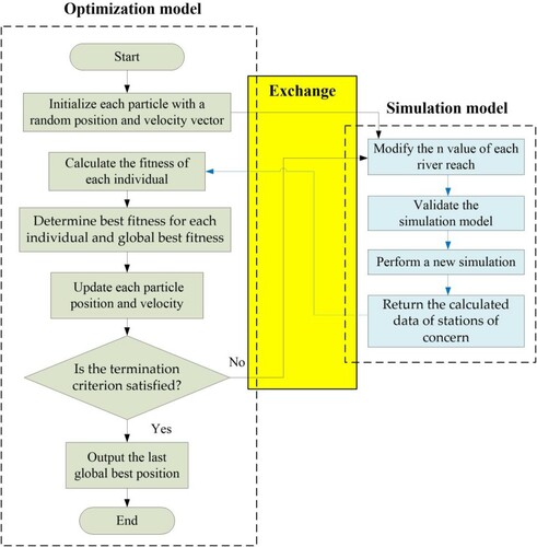
Figure 4. NSE probability density of each gauging station is indicated by the violin plot; the box plot and white point inside each violin plot indicate the interquartile range and the average of NSE, respectively. The red line with triangle markers indicates the SI calculated by Equation (10).

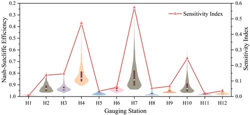
Figure 5. Spatial distribution of SI in study area as drawn using a kriging method with the calculated SI of each point in the simulation model.

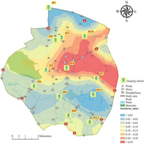
Figure 6. Gray line with blue triangles indicates fitness of each simulation. Each generation has 20 particles (realizations). Red line indicates global best fitness of each generation.

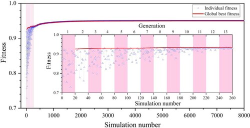
Figure 7. Individual performance during calibration. Blue triangles indicate NSE of each station for each simulation.

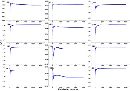
Figure 8. Calibration results for gauging stations. Red lines indicate best simulation results, and blue triangles indicate observed data.

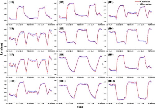
Table 4. Performance of optimization-simulation model for each gauging station. NSE, R, and PBIAS are shown for the best simulation.

	Gauging station
Criteria	H1	H2	H3	H4	H5	H6	H7	H8	H9	H10	H11	H12
NSE	0.990	0.966	0.964	0.898	0.983	0.975	0.935	0.989	0.973	0.963	0.978	0.985
R	0.995	0.983	0.982	0.950	0.993	0.988	0.967	0.995	0.987	0.982	0.994	0.993
PBIAS	0.35	−0.14	0.07	0.05	−0.78	−0.23	0.03	0.37	−0.22	0.03	−2.08	−0.42

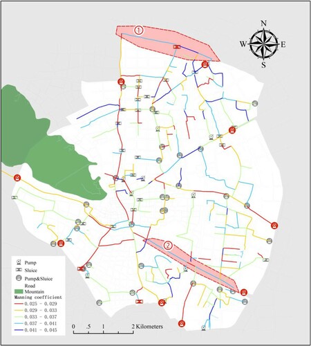
Figure 9. Spatial distribution of optimal Manning roughness coefficients as estimated using optimization-simulation model. Some river reaches with unreasonable roughness are marked by a red dotted line.