MAST-RT0 solution of the incompressible Navier–Stokes equations in 3D complex domains

Figures & data

Figure 1. RT0 kinematic pressure contour lines in the face common to two tetrahedrons.

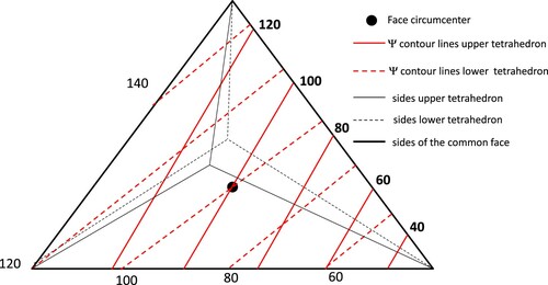
Figure 2. (a) The two tetrahedrons e and ep satisfy the EDP. (b) The two tetrahedrons do not satisfy the EDP.

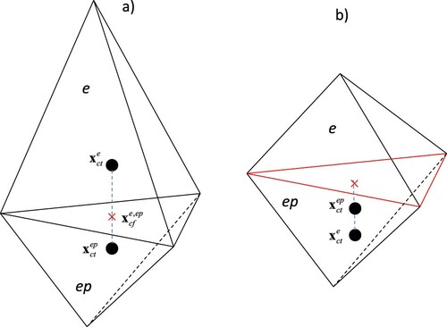
Figure 3. Sketch of MAST algorithm in the 1D case.

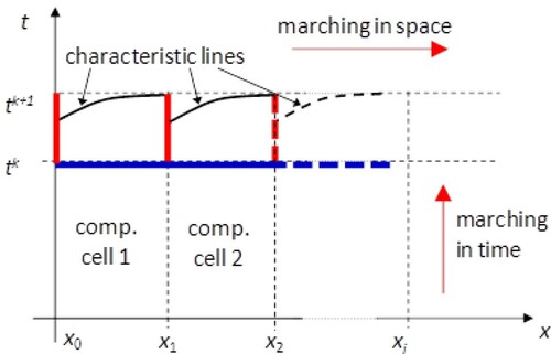
Figure 4. Solution of a single time step. (a) Scheme of the parallel solution of the MAST-fs (or MAST-bs). (b) Scheme of the parallel solution of traditional MArching in Time method (MTM).

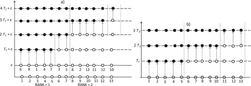
Figure 5. 1D sketch of velocity vectors inside tetrahedron e.

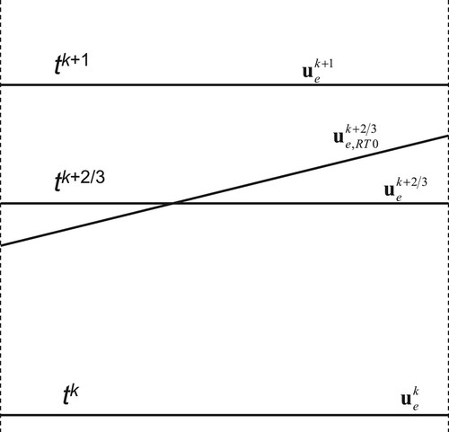
Figure 6. (a) 2D sketch of case $N_{f,m}^{\mathrm{int}}$ = N_T,m – 1. (b) 2D sketch case of $N_{f,m}^{\mathrm{int}}$ = N_T,m. Blue solid lines are traces of the external faces of the cluster, and red dashed lines are traces of the internal faces of the cluster.

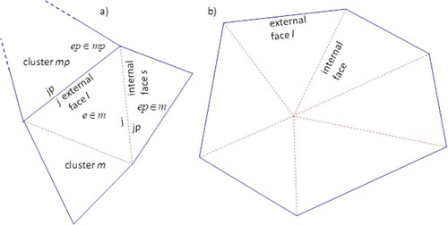
Table 1. Test 1. L₂ norms of relative errors and spatial rate of convergence.

hl [m]	L2 err u	L2 err v	L2 err ψ	rc,s u	rc,s v	rc,s ψ
6.60E–02	1.36E–02	1.37E–02	2.58E–02	–	–	–
2.47E–02	4.45E–03	4.47E–03	6.24E–03	1.14E+00	1.14E+00	1.45E+00
1.69E–02	2.82E–03	2.84E–03	3.50E–03	1.19E+00	1.18E+00	1.50E+00
1.28E–02	2.03E–03	2.05E–03	2.28E–03	1.18E+00	1.17E+00	1.55E+00
9.96E–03	1.50E–03	1.51E–03	1.53E–03	1.22E+00	1.21E+00	1.59E+00

Table 2. Test 1. L∞ norms of relative errors and spatial rate of convergence.

hl [m]	L∞ err u	L∞ err v	L∞ err ψ	rc,s u	rc,s v	rc,s ψ
6.60E–02	3.04E–02	3.07E–02	5.77E–02	–	–	–
2.47E–02	9.98E–03	1.00E–02	1.40E–02	1.13E+00	1.14E+00	1.44E+00
1.69E–02	6.32E–03	6.35E–03	7.85E–03	1.19E+00	1.18E+00	1.50E+00
1.28E–02	4.56E–03	4.59E–03	5.10E–03	1.18E+00	1.17E+00	1.55E+00
9.96E–03	3.37E–03	3.39E–03	3.44E–03	1.22E+00	1.21E+00	1.59E+00

Figure 7. Test 1. Iso-contours of the relative error of the norm of (a) u, (b) ψ.

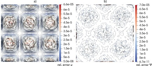
Figure 8. Test 1. Investigation of the spatial and temporal accuracy. (a) Norms of relative errors vs. mean mesh size, (b) norms of relative errors vs. time step size.

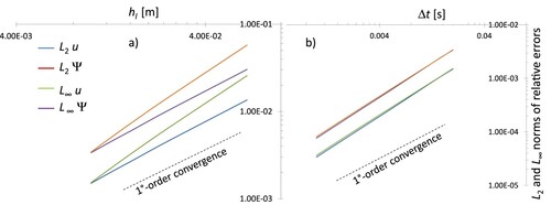
Table 3. Test 1. L₂ norms of relative errors and time rate of convergence.

Δt [s]	L2 err u	L2 err v	L2 err ψ	rc,t u	rc,t v	rc,t ψ
0.02	1.50E–03	1.51E–03	1.53E–03	–	–	–
0.015	1.06E–03	1.06E–03	1.07E–03	1.20E+00	1.22E+00	1.26E+00
0.01	6.33E–04	6.33E–04	6.47E–04	1.28E+00	1.28E+00	1.24E+00
0.005	2.60E–04	2.61E–04	2.74E–04	1.28E+00	1.28E+00	1.24E+00
0.0025	1.08E–04	1.08E–04	1.16E–04	1.26E+00	1.27E+00	1.25E+00
0.001	3.39E–05	3.45E–05	3.63E–05	1.27E+00	1.25E+00	1.27E+00

Table 4. Test 1. L∞ norms of relative errors and time rate of convergence.

Δt [s]	$L_{\mathrm{\infty }}$ err u	$L_{\mathrm{\infty }}$ err v	$L_{\mathrm{\infty }}$ err ψ	rc,t u	rc,t v	rc,t ψ
0.02	3.37E–03	3.39E–03	3.44E–03	–	–	–
0.015	2.39E–03	2.38E–03	2.39E–03	1.19E+00	1.22E+00	1.26E+00
0.01	1.42E–03	1.42E–03	1.45E–03	1.29E+00	1.28E+00	1.24E+00
0.005	5.83E–04	5.84E–04	6.15E–04	1.28E+00	1.28E+00	1.24E+00
0.0025	2.44E–04	2.43E–04	2.59E–04	1.26E+00	1.27E+00	1.25E+00
0.001	7.62E–05	7.73E–05	8.12E–05	1.27E+00	1.25E+00	1.27E+00

Figure 9. Test 1. Computational time of model steps.

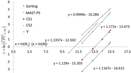
Figure 10. Test 2. (a) set-up of the numerical test and BCs. (b) section of the mesh with a cutting plane.

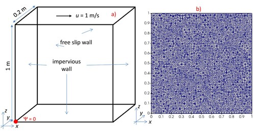
Figure 11. Test 2. Velocity streamlines (left panels), vorticity (ω_z) (central panels), iso (kinematic) pressure (right panels). Top Re = 100, middle Re = 400, bottom Re = 1000.

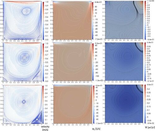
Figure 12. Test 2. x velocity component (top panel), z velocity component (bottom panel) (Nomenclature ‘Ref.’ are the results by Ghia et al. 1982).

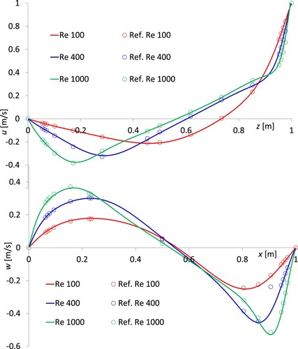
Figure 13. Test 3. Pattern of vortex shedding. Left panels Re = 300, (a) side view, (b) upper view. Right panel (c) 480 < Re < 800 (from Sakamoto & Haniu 1990)).

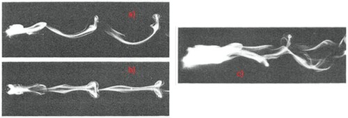
Figure 14. Test 3. (a) 3D view of the domain. (b) setup and BCs of the numerical runs.

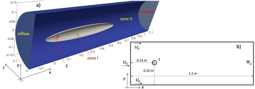
Figure 15. Test 3, Re = 300. Velocity streamlines in the (x–y) plane, stationary case.

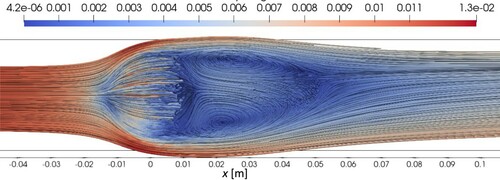
Table 5. Test 3. Values of the drag and lift coefficients.

	CD [–]		CL [–]
	Mean value	Amplitude value	Mean value	Amplitude value
Present solver without perturbation	0.67043	–	−0.0675	–
Present solver with perturbation (Equation (85))	0.6678	2.91E-03	−0.06061	1.47E-02
Ploumhans et al. (2002)	0.683	2.50E-03	−0.061	1.40E-02
Johnson and Patel (1999)	0.656	3.50E-03	−0.069	1.60E-02
Tomboulides (1993)	0.671	2.80E-03	not reported	not reported
Roos and Willmarth (1971)	0.629	not reported	not reported	not reported

Figure 16. Test 3, Re = 300. 3D periodic time evolution of the vortical structures.

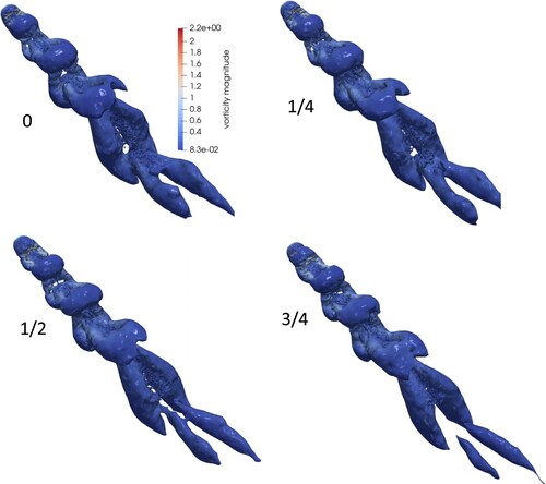
Figure 17. Test 3, Re = 300. Periodic time evolution of the velocity streamlines (left panels) and kinematic pressure (right panels), (x–z) plane.

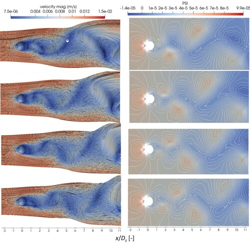
Figure 18. Test 3, Re = 300. Periodic time evolution of the velocity streamlines (left panels) and kinematic pressure (right panels), (x–y) plane.

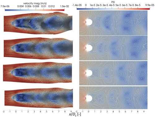
Figure 19. Test 3, Re = 600. (a) 3D vortical structure at τ* = 35. (b) Time evolution of the drag, lift and side coefficients.

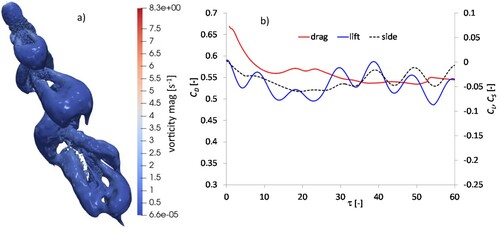
Table 6. MAST solution time vs. no. of processors.

Np	Tmin/TT	TMAST/TT	TMAST /Tmin
4	676,184,582	680,355,106	1.006
12	225,394,080	229,004,379	1.016
40	67,618,224	71,041,472	1.051
50	54,094,345	57,521,651	1.063
100	27,046,587	30,304,361	1.120
150	18,031,058	20,938,102	1.161
200	13,522,708	16,347,121	1.209
250	10,818,869	15,173,010	1.402

Figure 20. (a) Test 4. Real and computational domain. (b) computational mesh. (c) Section of the mesh with a generic plane.

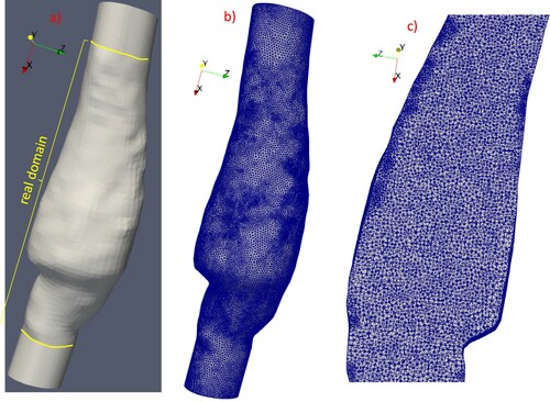
Figure 21. Test 4. (a) waveforms of mean-in-time inflow velocity and outlet pressure. (b) Womersley inflow velocity profiles at four significant times (from Aricò et al., 2020).

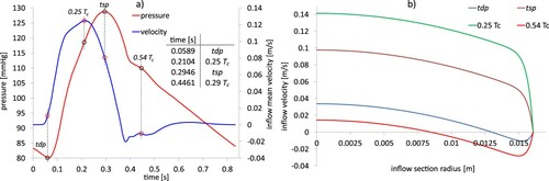
Figure 22. Test 4. Computed velocity vectors and kinematic pressure at the significant times in Figure 21.

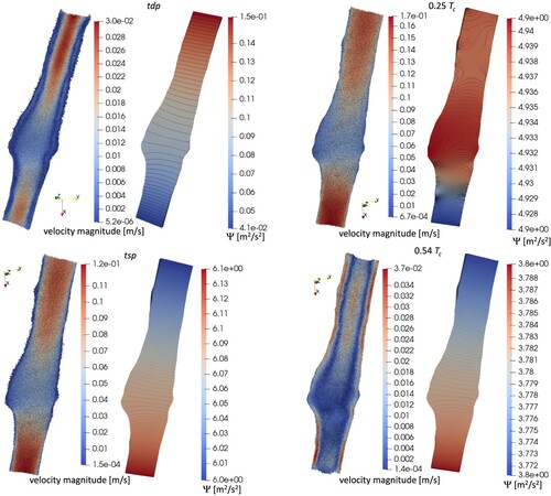
Figure 23. Test 4. Zoom of the velocity fields for tdp and 0.54 T_c.

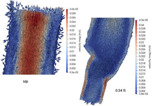
Figure 24. Test 4. Velocity components computed along the axis shown in Figure 25, for two meshes.

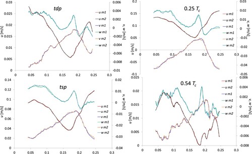
Figure 25. Test 4. Initial and final axis position.

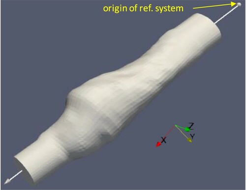
Figure A1. Flow-chart of the Order subroutine.

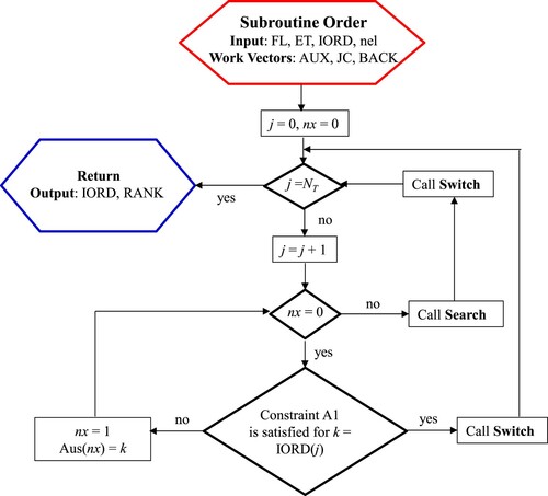
Figure A2. Flow-chart of the Search subroutine.

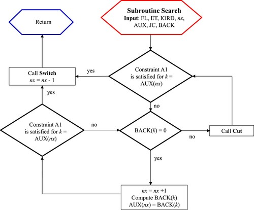
Figure A3. Flow-chart of the Cut subroutine.

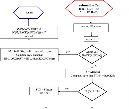
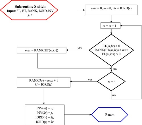
Figure A4. Flow-chart of the Switch subroutine.

Ghia, U., Ghia, K. N., & Shin, C. T. (1982). High-resolutions for incompressible flow using the Navier-Stokes equations and a multigrid method. Journal of Computational Physics, 48, 387–411. https://doi.org/https://doi.org/10.1016/0021-9991(82)90058-4

 Web of Science ®Google Scholar

Sakamoto, H., & Haniu, H. (1990). A study of vortex shedding from spheres in a uniform flow. Journal of Fluids Engineering, 112, 386. https://doi.org/https://doi.org/10.1115/1.2909415

 Web of Science ®Google Scholar

Ploumhans, P., Winckelmans, G. S., Salmon, J. K., Leonard, A., & Warren, M. S. (2002). Vortex methods for direct numerical simulation of three-dimensional bluff body flows: Application to the sphere at Re = 300, 500, and 1000. Journal of Computational Physics, 178, 427–463. https://doi.org/https://doi.org/10.1006/jcph.2002.7035

 Web of Science ®Google Scholar

Johnson, T. A., & Patel, V. C. (1999). Flow past a sphere up to a Reynolds number of 300. Journal of Fluid Mechanics, 378, 19–70. https://doi.org/https://doi.org/10.1017/S0022112098003206

 Web of Science ®Google Scholar

Tomboulides, A. G. (1993). Direct and Large-Eddy simulation of wake flows: Flow past a sphere, PhD thesis, Princeton University.

 Google Scholar

Roos, F. W., & Willmarth, W. W. (1971). Some experimental results on sphere and disk drag. AIAA Journal, 9, 285–291. https://doi.org/https://doi.org/10.2514/3.6164

 Web of Science ®Google Scholar

Aricò, C., Sinagra, M., Nagy, R., Napoli, E., & Tucciarelli, T. (2020). Investigation of the hemodynamic flow conditions and blood-induced stresses inside an abdominal aortic aneurysm by means of a SPH numerical model. International Journal for Numerical Methods in Biomedical Engineering, 36, 3263. https://doi.org/https://doi.org/10.1002/cnm.3263

 Web of Science ®Google Scholar