Numerical optimization of three-cavity magneto mercury reciprocating (MMR) micropump

Figures & data

Figure 1. The three-cavity MMR micropump.

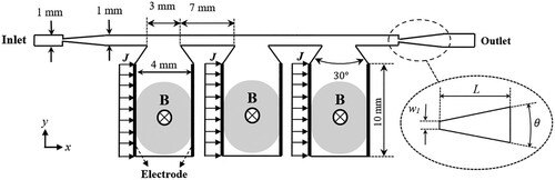
Table 1. The three-cavity MMR micropump variables.

Parameter	Value
B (T)	0.25
$I_0$ (A)	2
f (Hz)	10
s (mm)	8

Figure 2. A schematic of the three-cavity MMR micropump at the beginning of the four steps of a pump cycle.

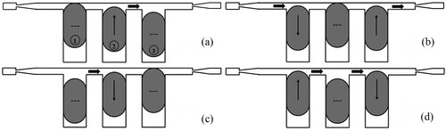
Figure 3. The electric current imposed to the (a) first, (b) second, and (c) third mercury slug during the four steps of the MMR micropump pumping cycle with $\mathrm{\Delta }\varphi ={90}^{\circ }$. When the current is in the $+x$ and $-x$ direction, it has a positive and negative sign, respectively.

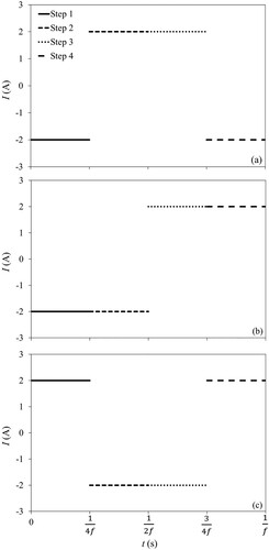
Table 2. Physical properties of air and mercury at ${25}^{\circ }\mathrm{C}$.

Property	Mercury	Air
$\rho (\mathrm{k}\mathrm{g}/{\mathrm{m}}^3$)	13,567	0.1855
$\mu (\mathrm{P}\mathrm{a}.\mathrm{s})$	$1.52\times {10}^{-3}$	$1.85\times {10}^{-5}$
$\sigma \left(\mathrm{N}/\mathrm{m}\right)$	0.4855
$\theta {}_{\mathrm{s}}{(}^{\circ })$	135

Figure 4. The volume fraction contours, where the red and blue colors represent volume fractions of 1 (mercury) and 0 (air), respectively, for the four cases with (a) 17,880, (b) 40,302, (c) 72,100, and (d) 161,790 number of cells.

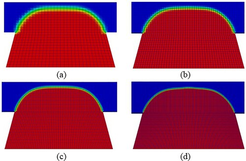
Table 3. Computational grid sensitivity study data.

Case	Number of cells	Mean pumping flow rate (mL/min)	The differences in flow rate (%)
1	17,880	9.15	−
2	40,302	8.50	7.6
3	72,100	8.15	4.3
4	161,790	8.04	1.4

Table 4. The micropump mean pumping flow rate predictions based on different maximum Courant numbers.

Case	Maximum allowable Courant number	The mean pumping flow rate (mL/min)	The differences in the flow rates (%)
1	1	7.68	–
2	0.4	8.13	5.54
3	0.2	8.15	0.25

Figure 5. (a) The comparison of the MMR micropump pumping flow rate estimated by the numerical estimations with the experimental measurements (Karmozdi et al., 2013) at different back-pressures. (b) A schematic of a mercury slug in a rectangular channel.

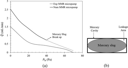
Table 5. The experimental prototype variables.

Parameter	Value
B (T)	0.2
$I_0$ (A)	1.5
f (Hz)	9
$\mathrm{\Delta }\varphi$ (${}^{\circ }$)	90
s (mm)	2

Figure 6. The comparison of the outlet flow rate of the MMR micropump with an excitation frequency of 10 Hz at a back-pressure of 10 Pa when the phase difference value is 90${}^{\circ }$ and 120${}^{\circ }$.

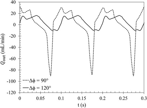
Figure 7. The variation of the mean flow rate of the MMR micropump with an excitation frequency of 10 Hz at a back-pressure of 10 Pa as a function of the electric current phase difference.

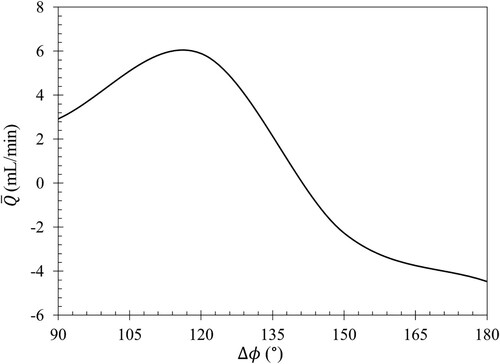
Figure 8. The mercury slugs configuration during the operation of the micropump with a frequency of 10 Hz and a phase difference of 30${}^{\circ }$ at a back-pressure of 10 Pa.

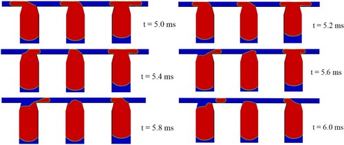
Figure 9. A snapshot at 0.14 s of the pressure contours of the micropump with a frequency of 10 Hz and a phase difference of 120${}^{\circ }$ at a back-pressure of 30 Pa.

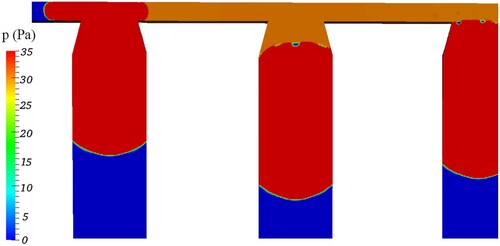
Figure 10. The time evolution of the outlet flow rate of the three-cavity MMR micropump with a phase difference of (a) 90${}^{\circ }$ and (b) 120${}^{\circ }$ and an excitation frequency of 10 Hz as a function of back-pressure.

Figure 11. The mean flow rate of the micropump with an excitation frequency of 10 Hz as a function of the back-pressure for phase differences of 90${}^{\circ }$ and 120${}^{\circ }$.

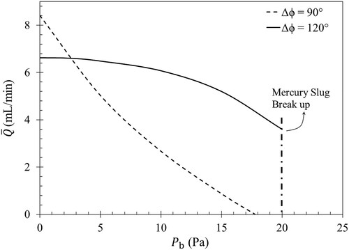
Table 6. The mean reverse flow rate of diffuser/nozzle valves at a back-pressure of 1.2 Pa as a function of their length and angle.

Case	L (mm)	θ (${}^{\circ }$)	Mean reverse flow rate (mL/min)
1	1	10	31.76
2	1	46	3.19
3	2.5	10	15.34
4	2.5	20	0.97
5	4	10	4.58
6	4	12	1.54
7	5	7	6.11
8	5	10	0.83
9	6	8.2	0.87

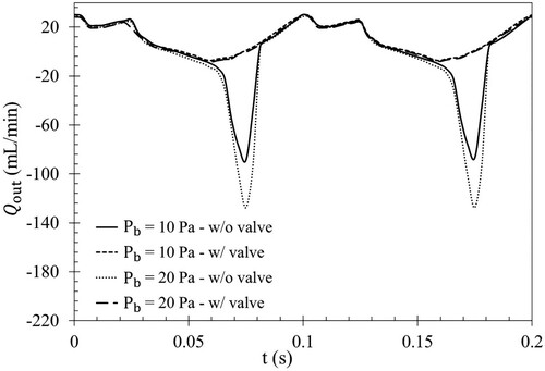
Figure 12. Comparison of three-cavity MMR micropump with and without the diffuser/nozzle valve in frequency of 10 Hz and phase difference of 90${}^{\circ }$.

Karmozdi M., Salari A., & Shafii M. B. (2013). Experimental study of a novel magneto mercury reciprocating (MMR) micropump, fabrication and operation. Sensors and Actuators A: Physical, 194, 277–284. https://doi.org/https://doi.org/10.1016/j.sna.2013.02.012

 Web of Science ®Google Scholar