Insight into dust control performance of a reverse circulation drill bit using multiphase flow simulation

Figures & data

Figure 1. Dust explosion of conventional DTH air hammer drilling (left) and fine dust control performance of reverse circulation DTH air hammer drilling (right).

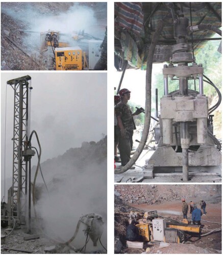
Figure 2. Schematic diagram of reverse circulation drilling system.

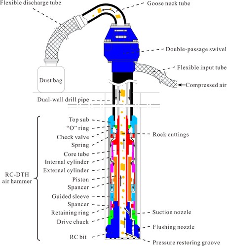
Table 1. Analysis of grid sensitivity and grid type.

Grid		Number of cells	Qent (kg/s)
Hexahedral cells		181,784	0.024401247
Polyhedral cells	Fine grid	306,231	0.023962019
	Medium grid	585,867	0.025249742
	Coarse grid	908,714	0.025369412
%Difference			5.8

Figure 3. (a) Influence of air compressibility on the suction capacity. (b) Influence of the input air volume flow rate using compressible air (ideal gas) on suction capacity.

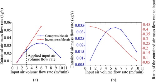
Table 2. Part of parameters used in the simulations.

Parameter	Value	Investigated parameter	Value(variable)
Gravity acceleration (m/s^2)	−9.81 (Y direction)	Volume flow rate(m^3/min)	3 (1∼3)
Air Density (kg/m^3)	1.225	Rotary Speed(rpm)	0 (0∼60)
Viscosity (kg/m/s)	$1.79\times {10}^{-5}$	Feed concentration (%)	20 (10∼30)
Density of granular (kg/m^3)	2650	ROP (m/h)	10 (10∼30)
		Granular diameter (mm)	3 (1∼9)
		Specularity Coefficient	0.01 (0.01∼0.2)

Figure 4. Typical grid model and boundary conditions of computational domain.

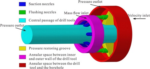
Figure 5. Schematic diagram of the RC-bit flow field.

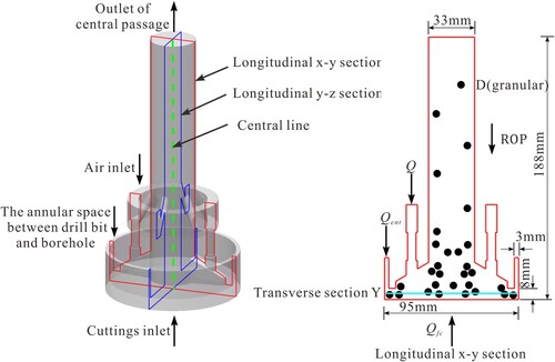
Figure 6. Typical distribution of cuttings: (a) volume fraction contour plot of X-Y section, (b) streamline distribution plot of X-Y section, (c) volume rendering of isometric view, (d) volume fraction contour plot of bottom borehole, and (e) streamline distribution plot of bottom borehole.

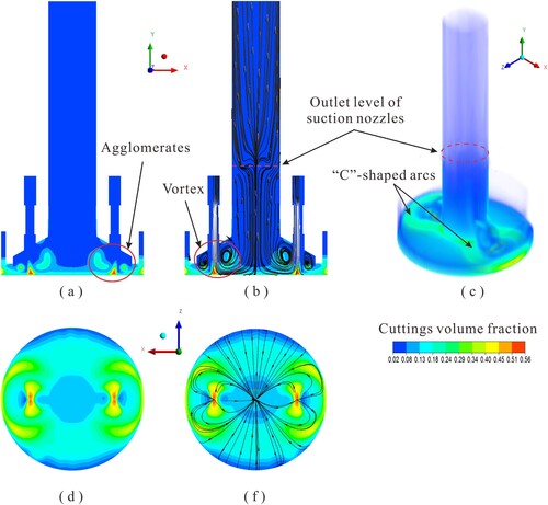
Figure 7. Contour plots of cuttings volume fraction.

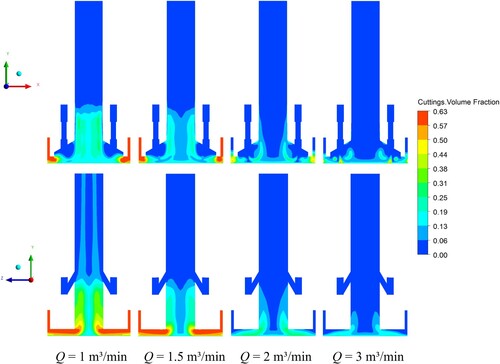
Figure 8. (a) Effect of the input air volume flow rate on the suction capacity. The negative values represent the air released to the atmosphere from the annular gap. (b) Static pressure distribution along the centerline.

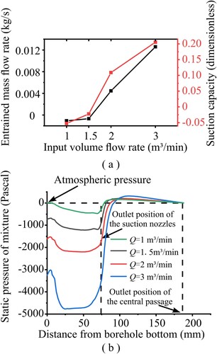
Figure 9. Effect of rotary speed on the suction capacity (Q = 3 m³/min).

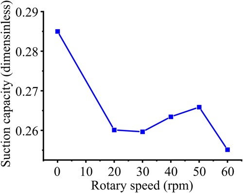
Figure 10. Volume fraction contour plots showing the distribution of cutting particles with different rotary speed (Y = 2 mm).

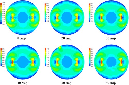
Figure 11. Volume fraction line plots showing the distribution of cutting particles in radial position with different rotary speed (Y = 2 mm).

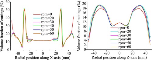
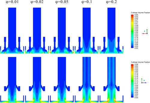
Figure 12. Volume fraction contour plots showing the distribution of cutting particles with different feed concentration: (a) Y = 2 mm, (b) Y = 4 mm, (c) Y = 6 mm, (d) X-Y section.

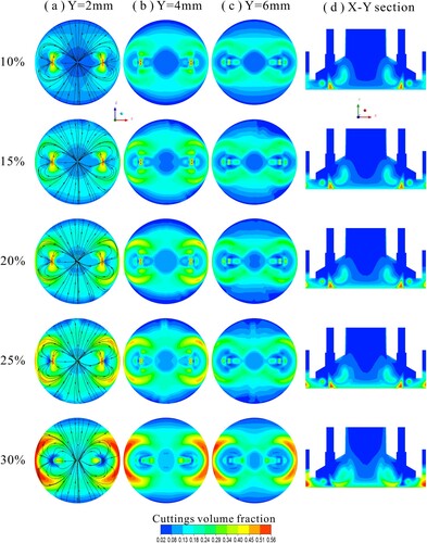
Figure 13. Effect of volume fraction of cuttings on the suction capacity.

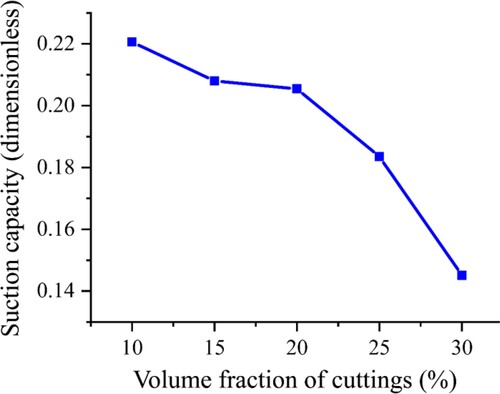
Figure 14. Volume fraction contour plots showing the distribution of cutting particles with a distance of 2 mm from bottom. (a) ROP = 10 m/h, (b) ROP = 15 m/h, (c) ROP = 20 m/h, (d) ROP = 25 m/h, and (e) ROP = 30 m/h. Line plot (f) showing the impact of ROP on suction capacity.

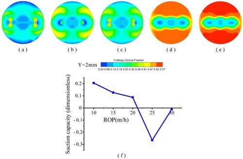
Figure 15. Effect of diameter of cuttings on the suction capacity.

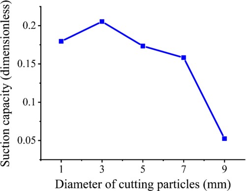
Figure 16. Velocity of cuttings with different diameters on the central line of central passage.

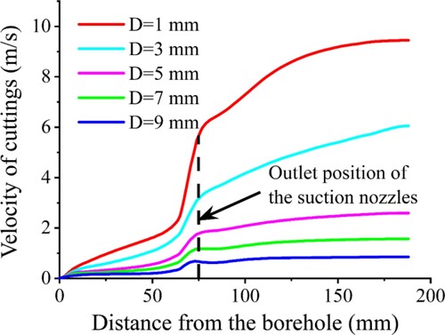
Figure 17. Effect of specularity coefficient on the suction capacity.

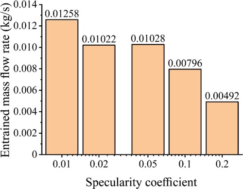
Figure 18. Volume fraction contour plots showing the distribution of cutting particles.