Figures & data
Figure 1. Possible techniques to create volume meshes from CT data. Performing a CT scan generates an image stack with grey values. The approaches presented in literature are divided into direct and indirect methods. While approaches from the first method directly create volume meshes out of CT data, the indirect methods process the CT data to create a surface mesh and additional software has to be used for creating the volume meshes. Detailed descriptions: The first approach generates cubes out of the voxels, while the second approach (Volumetric Marching Cubes, VoMaC) uses the Marching Cubes (MC) algorithm as a basis. The third approach utilizes Non-Uniform Rational B-Splines (NURBS) to represent the contours, the fourth approach is the classical MC algorithm, and the fifth approach works with a point cloud based on grey prediction (GP) modelling.
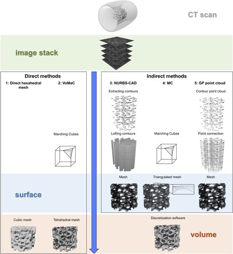
Figure 2. Schematic of the workflow from the physical object to the final volume mesh. The investigated objects are a sphere, a POCS and a 10 and 20 ppi OCF. The surface mesh represents the geometry, which is the basis for volume mesh generation. The process steps are performed with ImageJ (I), ParaView (II), Blender (III) and OpenFOAM (IV). All scale bars represent 5 mm.
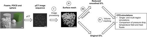
Table 1. Morphological properties of the investigatedgeometries.
Figure 3. Overview of the simulation area and the main boundary conditions for single-region (SR) and multi-region (MR) simulations.
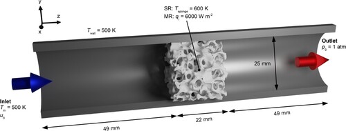
Figure 4. Influence of the process steps on the simple sphere geometry (diameter 1.2 cm, material alumina). (A) View onto the surface after surface reconstruction (STL generation). (B) View onto the surface after processing of STL. (C) Volume of the sphere at every consecutive process step normalised by the real value. (D) Surface of the sphere at every consecutive process step normalised with the real values. Dark blue indicates the original (unbinned) data whereas light blue indicates the binned data.
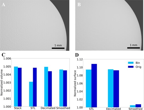
Figure 5. Influence of the processing steps on the POCS geometry (3D printed). (A) View onto struts after surface reconstruction (STL generation). (B) View onto the struts after processing of the STL. (C) Volume of the POCS at every consecutive process step normalised by the value of the digital parent. (D) Surface of the POCS at every consecutive process step normalised by the value of the digital parent. Dark orange indicates the original (unbinned) data whereas light orange indicates the binned data.
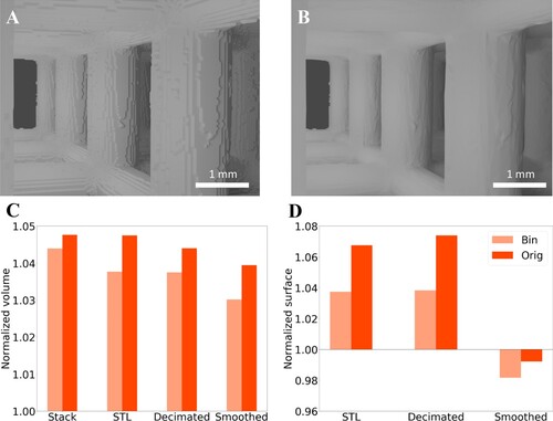
Figure 6. View onto a crossing point of the POCS’ struts. (A) Orthographic projection of the reconstructed POCS (yellow) superimposed on the digital parent (black). (B) Reflected-light microscope image, confirming the manufacturing process causes the differences between reconstructed POCS and digital parent.
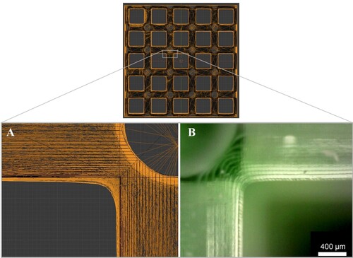
Figure 7. Influence of the processing steps on the OCF geometry (diameter 2.5 cm). (A) View onto the surface of the 10 ppi OCF after surface reconstruction (STL-generation). (B) View onto the surface of the 10 ppi OCF after processing of STL. (C) Volume of the OCFs at every consecutive process step normalised with the stack values. (D) Surface of the OCFs at every consecutive process step normalised with the STL values. Dark green indicates the 10 ppi OCF whereas light green indicates the 20 ppi OCF. All the data was gained from the binned image stacks.
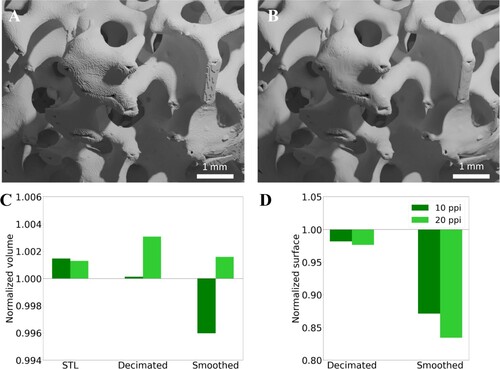
Figure 8. Superimposition of the binned 10 ppi sample without (red, 1.3 GB) and with (white, 130 MB) decimation and smoothing performed. The processing steps reduce the stepped surface appearance while preserving the overall geometry.
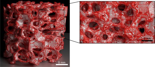
Table 2. Required memory size for the individual data files.
Figure 9. Meshing time (A) and RAM usage (B) for mesh UP and mesh P. Both for single- and multi-region meshes, the smoothed mesh reduces meshing time and RAM usage significantly.
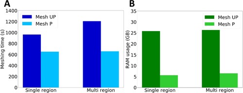
Figure 10. Single-region simulations. (A) Wall heat flux at a section of the OCF for mesh UP. (B) Wall heat flux at a section of the OCF for mesh P. Heat flux is given in W m−2 at 0.5 m s−1 inlet velocity.
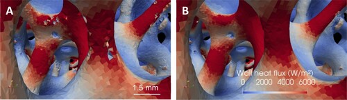
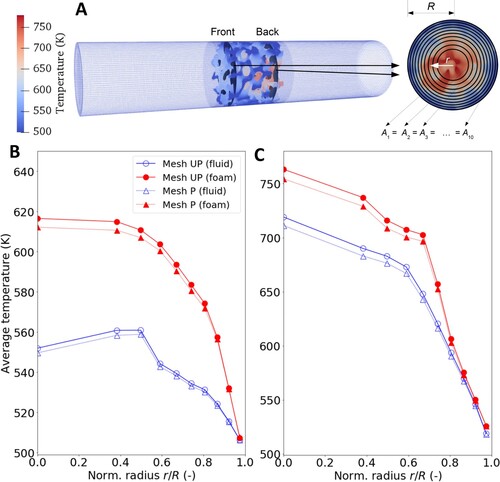
Figure 11. Radial averaging of temperature. (A) Illustration of the temperature analysis method. Two slides are located 3 mm downstream of the beginning (front) and 3 mm upstream of the end of the OCF (back). 10 annuli with equal areas were used to perform a radial averaging of the temperatures. (B) Radial temperature distribution in the front slice for the two different meshes. (C) Radial temperature distribution in the back slice for the two different meshes (evaluation method similar to Sinn et al., Citation2020).