Hydrodynamic performance of a rim-driven thruster improved with gap geometry adjustment

Figures & data

Figure 1. Geometry of the hubless RDT.

Table 1. Parameters of the RDT model.

Parameter	Unit	Value
Number of blades ($Z$)	–	4
Blade diameter ($D_b$)	m	0.25
Blade area ratio (${\lambda }_a$)	–	0.7
Blade pitch ratio (${\lambda }_p$)	–	1.0
Blade tip diameter ($D_t$)	m	0.05
Duct diameter ($D_d$)	m	0.3
Duct length ($L_d$)	m	0.125
Rim thickness ($H$)	m	0.006
Gap width ($S$)	m	0.0015

Figure 2. Geometric parameters of the gap.

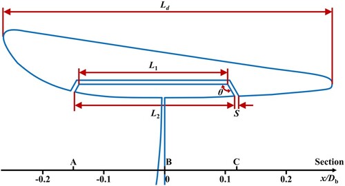
Figure 3. Computational domain and boundary conditions.

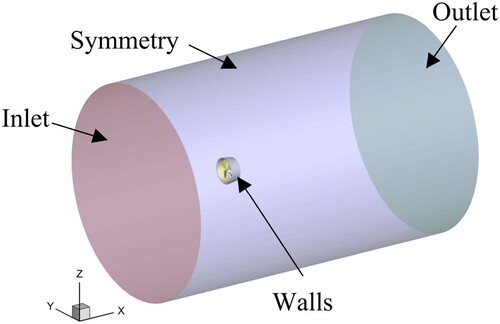
Figure 4. Mesh distribution: (a) surface mesh, (b) boundary layer, and (c) cells in the gap.

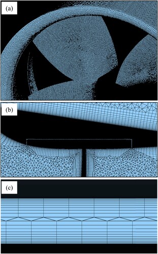
Table 2. Results of the grid convergence analysis.

	Total number of cells (millions)	$K_T$	GCI (%)	10$K_Q$	GCI (%)
Coarse	8	0.243	–	0.468	–
Medium	12	0.249	3.09	0.479	2.94
Fine	18	0.251	1.00	0.475	1.04

Figure 5. Comparison of open water characteristics between CFD and experimental results.

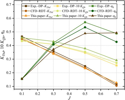
Figure 6. Hydrodynamic characteristics of the RDT at different oblique angles ($\theta$) with a fixed axial segment length of the gap.

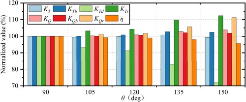
Figure 7. The axial velocity distribution of the flow field at different oblique angles ($\theta$) with a fixed axial segment length of the gap: (a) $\theta$ = 90°, (b) $\theta$ = 105°, (c) $\theta$ = 120°, (d) $\theta$ = 135°, and (e) $\theta$ = 150°.

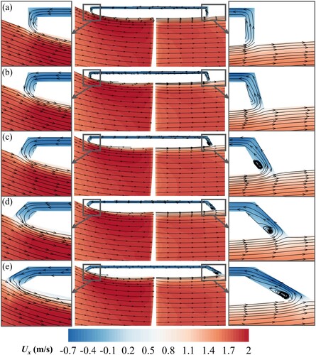
Figure 8. The pressure distribution of the flow field at different oblique angles ($\theta$) with a fixed axial segment length of the gap: (a) $\theta$ = 90°, (b) $\theta$ = 120°, and (c) $\theta$ = 150°.

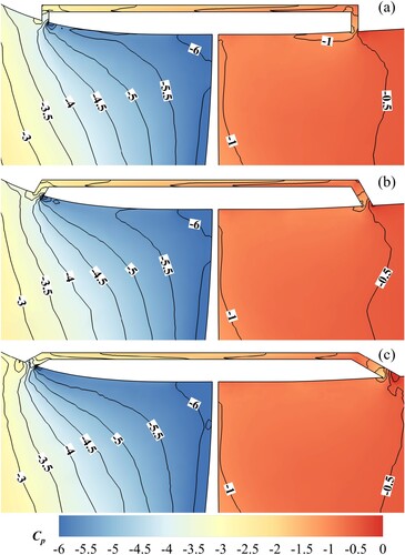
Figure 9. 3D pathlines in the gap at different oblique angles ($\theta$) with a fixed axial segment length of the gap: (a) $\theta$ = 90°, and (b) $\theta$ = 120°.

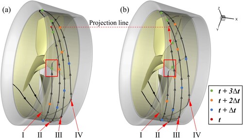
Figure 10. Hydrodynamic characteristics of the RDT at different oblique angles ($\theta$) with the fixed distance between the gap inlet and outlet.

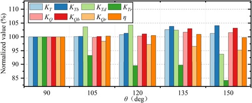
Figure 11. The axial velocity distribution of the flow field at different oblique angles ($\theta$) with the fixed distance between the gap inlet and outlet: (a) $\theta$ = 105°, (b) $\theta$ = 120°, (c) $\theta$ = 135°, and (d) $\theta$ = 150°.

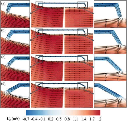
Figure 12. The dimensionless axial velocity contour distribution at different oblique angles ($\theta$ = 90° colored by red and $\theta$ = 135° colored by blue) with the fixed distance between the gap inlet and outlet: (a) cross section A, (b) cross section B, and (c) cross section C.

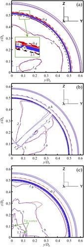
Figure 13. Vortex distribution visualized with an isosurface of the instantaneous Q-criterion in the wake field for the fixed inlet and outlet positions of the gap with different corner angles: (a) $\theta$ = 90°, and (b) $\theta$ = 135°.

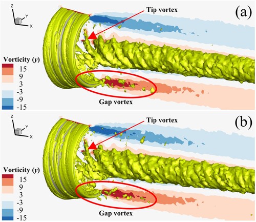
Figure 14. Gap vortex distribution visualized with an isosurface of the instantaneous Q-criterion in the wake field when $\theta$ = 90°.

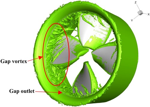
Figure 15. Positions and angles of the monitoring points located at the quarter-gap inlet and outlet.

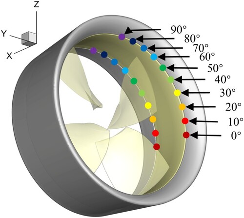
Figure 16. Pressure coefficient ($C_p$) curves at different monitoring points at different oblique angles ($\theta$) with the fixed distance between the gap inlet and outlet: (a) $C_p$ of the gap outlet, (b) $C_p$ of the gap inlet, and (c) relative $C_p$ between the inlet and outlet of the gap.

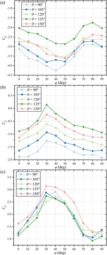
Figure 17. Value of the difference in pressure coefficients for the results of fixed $L_1$ ($C_{P1}$) and fixed $L_2$ ($C_{P2}$) at different monitoring points at different oblique angles ($\theta$): (a) the gap outlet, and (b) the gap inlet.

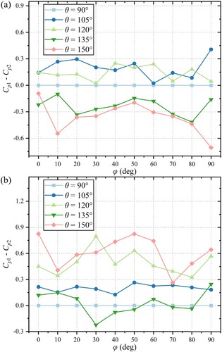
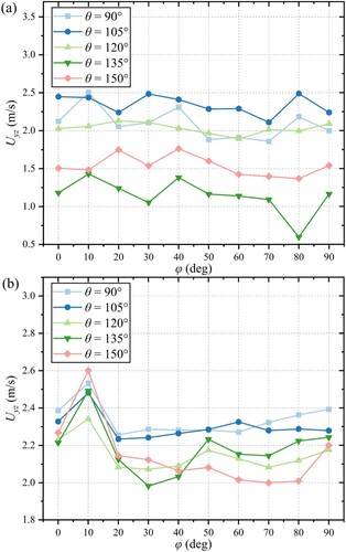
Figure 18. Axial velocities ($U_x$) of different monitoring points at different oblique angles ($\theta$) with the fixed distance between the gap inlet and outlet: (a) $U_x$ of the gap outlet, and (b) $U_x$ of the gap inlet.

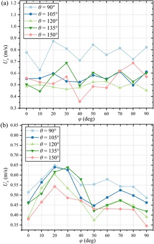
Figure 19. Combined velocities ($U_{yz}$) of different monitoring points on cross sections at different oblique angles ($\theta$) with the fixed distance between the gap inlet and outlet: (a) $U_{yz}$ of the gap outlet, and (b) $U_{yz}$ of the gap inlet.