Impact of the train heights on the aerodynamic behaviour of a high-speed train

Figures & data

Figure 1. Single-decker train and duplex-decker train: (a). TGV POS (Paris-Ostfrankreich-Süddeutschland) train and (b) TGV Duplex train. For more parameter details of the models, please refer to Masson et al. (2012) and Paradot and Bouchet (2009).

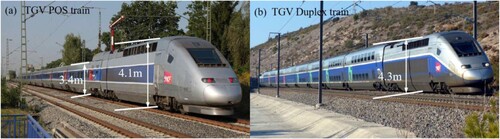
Figure 2. Train models: (a) front and overall elevation, (b) side elevation, and (c) vertical view (unit: mm).

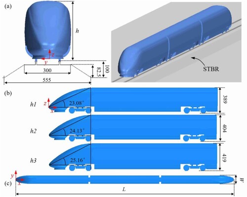
Figure 3. Schematic diagram of calculation domain and boundary.

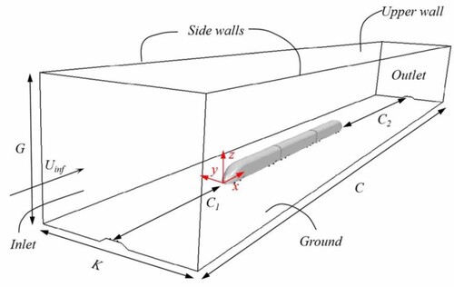
Table 1. The geometric size of the calculation domain and the train.

H	L	C	C1	C2	K	G
1.32W	26W	76W	15W	35W	40W	20W

Figure 4. The specific distribution of the medium grid: (a) vertical view and (b) lateral view. Grids details of the prism layers: (c) train upper surface and (d) bogie surface.

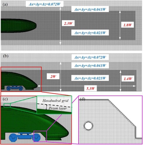
Table 2. Setting strategy of grid spatial scale for the h1 case.

Grids	$n_{mean}^{+}$	$n_{max}^{+}$	$\mathrm{\Delta }{s}_{mean}^{+}$	$\mathrm{\Delta }{s}_{max}^{+}$	$\mathrm{\Delta }{l}_{mean}^{+}$	$\mathrm{\Delta }{l}_{max}^{+}$	Size
Coarse	< 1.0	2.2	< 150	340	< 150	340	26 million
Medium	< 1.0	2.2	< 110	220	< 110	220	47 million
Fine	< 1.0	2.2	< 80	160	< 80	160	64 million

Figure 5. Comparison of calculation data for three grids: (a) time-average slipstream at the trackside location, (b) time-average slipstream at platform location, (c) time average velocity behind the train, and (d) aerodynamic drag and lift coefficient.

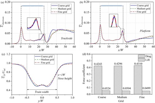
Figure 6. Verification of pressure coefficient (C_p) of the upper surface centreline of train: (a) head train and (b) tail train.

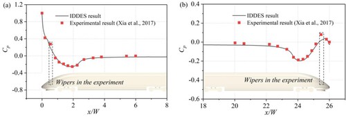
Figure 7. Slipstream verification at trackside location: (a) assemble-averaged slipstreams and (b) the curves of the standard deviation.

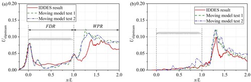
Table 3. Drag force and drag force coefficient.

	Cd						Fd (N)
	Mean			$\sigma$			Mean
Carriage	h1	h2	h3	h1	h2	h3	h1	h2	h3
Head	0.1620	0.1588	0.1551	0.0055	0.0048	0.0051	1.8424	1.8840	1.9216
Middle	0.1016	0.1004	0.0995	0.0044	0.0039	0.0039	1.1555	1.1905	1.2330
Tail	0.1660	0.1667	0.1641	0.0084	0.0076	0.0072	1.8879	1.9775	2.0333
Total	0.4296	0.4259	0.4188	0.0182	0.0163	0.0162	4.8858	5.0520	5.1878

Table 4. Lift force and lift force coefficient.

	Cl						Fl (N)
	Mean			$\sigma$			Mean
Carriage	h1	h2	h3	h1	h2	h3	h1	h2	h3
Head	−0.0415	−0.0419	−0.0434	0.0083	0.0060	0.0066	−0.4719	−0.4969	−0.5371
Middle	0.0019	0.0031	0.0034	0.0068	0.0060	0.0072	0.0212	0.0372	0.0417
Tail	0.0901	0.0939	0.0973	0.0116	0.0127	0.0120	1.0241	1.1143	1.2053
Total	0.0504	0.0552	0.0573	0.0267	0.0247	0.0257	0.5734	0.6546	0.7100

Figure 8. Surface pressure distribution under three train heights: (a) the pressure distributions at the upper centreline of the head train, (b) the pressure distributions at the upper centreline of the tail train, and (c) surface pressure distributions. The train is superimposed by the mean pressure coefficient.

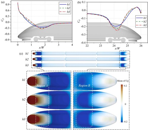
Figure 9. The PSD of the tail train forces: (a) drag force coefficients, (b) lift force coefficients.

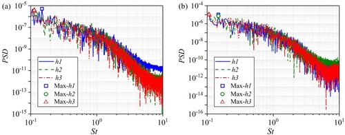
Figure 10. Comparison of the time-averaged slipstream along the sampled lines at 2.5, 3, and 3.5 m from the COT.

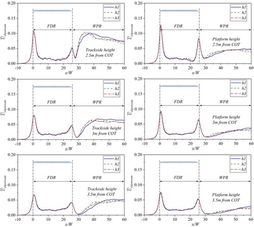
Figure 11. Comparison of peak time-averaged slipstreams for three cases: (a) Trackside locations, (b) Platform locations.

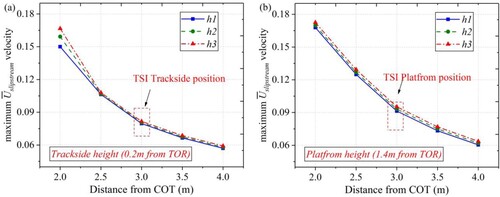
Figure 12. The boundary layer thickness of different sections. The sketch is coloured by mean velocity for the whole view and coloured by synthetic spanwise and vertical velocity for the cross-sections.

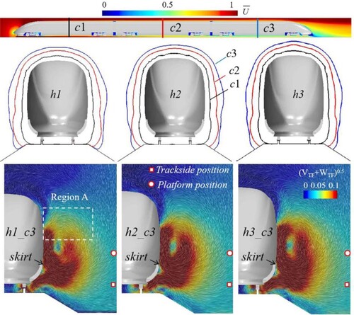
Figure 13. Instantaneous slipstreams. h1: (a) trackside location and (b) platform location. h2: (c) trackside location and (d) platform location. h3: (e) trackside location and (f) platform location.

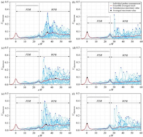
Figure 14. Schematic diagrams of instantaneous slipstream and iso-surfaces (Q = 10000) of z = 0.15W plane. The photograph is recorded at 350T_inf.

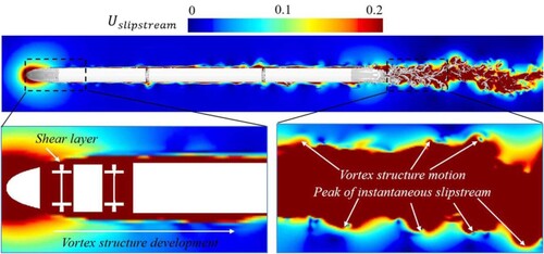
Figure 15. The 1s-average values of instantaneous slipstreams. h1: (a) trackside location and (b) platform location. h2: (c) trackside location and (d) platform location. h3: (e) trackside location and (f) platform location.

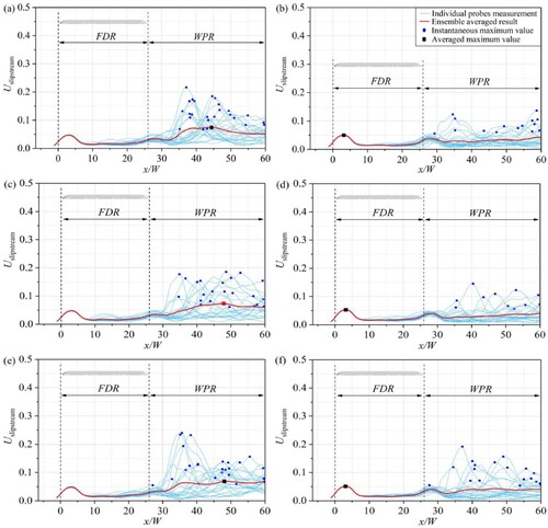
Table 5. Amplitude statistics of the instantaneous slipstreams with or without the 1s-average method.

		Without 1s-average			With 1s-average
Locations	Train heights	${\overline{U}}_p$	σ	$U_{TSI}$	${\overline{U}}_p$	σ	$U_{TSI}$
Trackside	h1	0.1785	0.0619	0.3023	0.1073	0.0342	0.1757
	h2	0.1878	0.0694	0.3266	0.1091	0.0360	0.1811
	h3	0.1971	0.0770	0.3511	0.1146	0.0371	0.1888
Platform	h1	0.1196	0.0354	0.1904	0.0680	0.0291	0.1262
	h2	0.1264	0.0467	0.2198	0.0694	0.0293	0.1280
	h3	0.1392	0.0487	0.2366	0.0706	0.0296	0.1298

Figure 16. Surface flow diagram of the tail train. The train surface is coloured by the time-averaged wall shear stress.

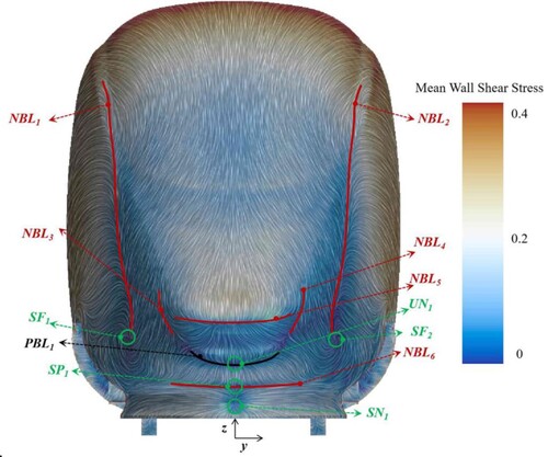
Figure 17. Spanwise vortices and velocity distribution in the WPR: (a) Spanwise vortices and (b) velocities sampled along vertical lines.

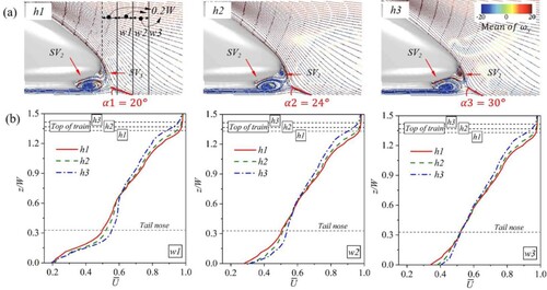
Figure 18. Instantaneous iso-surfaces coloured by vorticity magnitude (Q = 12000). The photographs are recorded at 350T_inf.

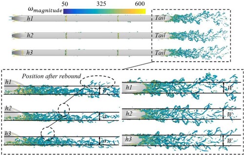
Figure 19. Spatial streamline at different train heights. The train is superimposed by the time-average pressure coefficient.

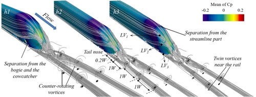
Figure 20. Spatial distribution of vortex cores: (a) The spatial distribution of the vortex cores and the cross-sectional tail streamlines; (b) variation of vortex core width with train height; (c) variation of the average height of vortex core with train height.

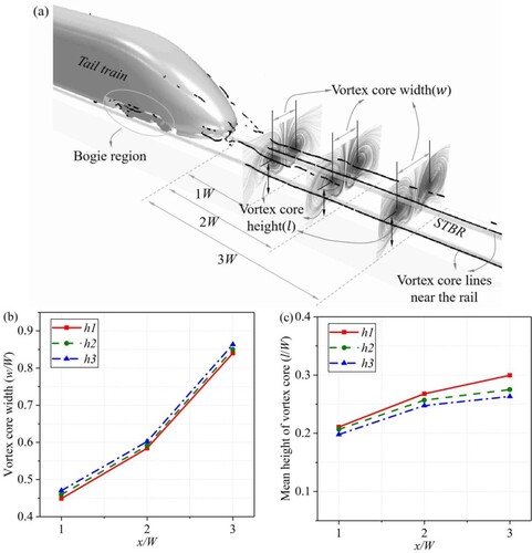
Figure 21. The development stage of the tail streamlines and quantitative analysis of the characteristic lengths of the vortex cores.

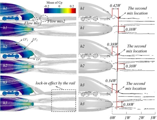
Figure 22. Distribution of mean slipstreams in three cases: (a) Comparison of slipstream velocities on three vertical planes in WPR, (b) comparison of slipstream isopleth (0.2, 0.3, and 0.4) in three cases, and (c) comparison of slipstream velocities in flow direction plane.

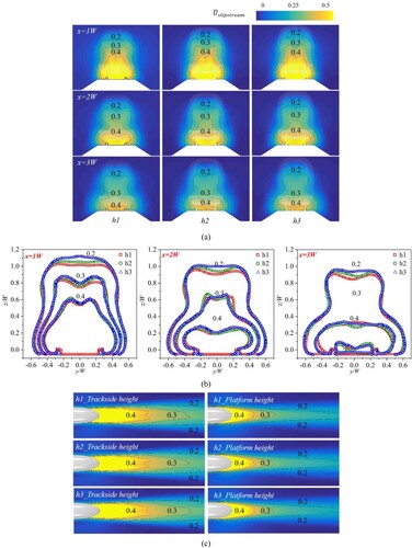
Figure 23. Safety analysis of CEN Standard for slipstream velocities: (a) Time-averaged slipstreams, and (b) TSI slipstreams with the 1s-average method.

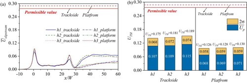
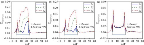
Figure 24. Comparison of time-averaged slipstreams on top of trains at y = 0 plane for three cases: (a) 4.3 m (full scale) from the TOR, (b) 4.5 m from the TOR, and (c) 5 m from the TOR.

Masson, E., Paradot, N., & Allain, E. (2012). Notes on numerical fluid mechanics and multidisciplinary design. Noise and Vibration Mitigation for Rail Transportation Systems, 118(5), 437–444. https://doi.org/10.1007/978-4-431-53927-8_52

 Google Scholar

Paradot, N., & Bouchet, J. P. (2009). Determination of aerodynamic coefficients of the TGV Duplex in wind tunnel for flat ground configurations. EuroMech colloquium 509, Vehicle Aerodynamics, Berlin, Germany.

 Google Scholar

Data availability

The data that supports the findings of this study are available from both the first author and the corresponding author upon reasonable request.