Analysis of cavitation and shear in bellows pump: transient CFD modelling and high-speed visualization

Figures & data

Figure 1. Sketch of a pneumatic drive bellows pump (PDBP).

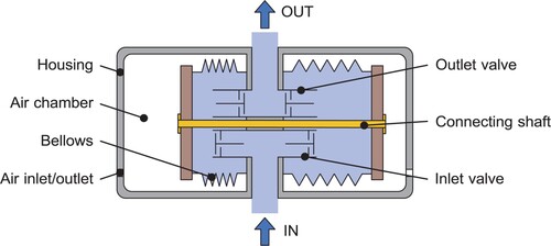
Figure 2. (a) Schematic overview of the experimental system. 1-water tank, 2,8-ball valve, 3,7-flow meter, 4,6-pressure sensor, 5-test pump, 9-thermal sensor, 10-data acquisition card, 11-computer, 12-air source, 13-switch, 14-pressure regulator, 15-solenoid on-off valve, 16-solenoid directional valve, 17,18-silencer, 19,20-quick exhaust valve, 21-cylinder, 22-laser displacement sensor. (b) Photography of the test pump containing a close-up view of the check valve at the bottom left.

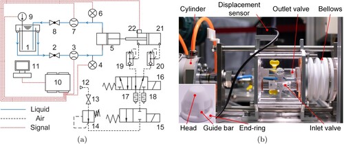
Table 1. Geometrical parameters of the test pump.

Parameter	Symbol	Value	Unit
Diameter of inlet (or outlet) pipe (or channel)	d	16.0	$\mathrm{m}\mathrm{m}$
Outer diameter of the bellows	$D_{\mathrm{b}}$	110.5	$\mathrm{m}\mathrm{m}$
Inner diameter of the bellows	$d_{\mathrm{b}}$	76.5	$\mathrm{m}\mathrm{m}$
Effective diameter of the bellows	$d_{\mathrm{b}\mathrm{e}}$	95.0	$\mathrm{m}\mathrm{m}$
Cone angle of check valves	β	60.0	${}^{\circ }$
Outer diameter of check valves	$D_{\mathrm{v}}$	22.5	$\mathrm{m}\mathrm{m}$
Diameter of valve cases	$d_{\mathrm{v}\mathrm{c}}$	24.0	$\mathrm{m}\mathrm{m}$
Axial length of check valves	$L_{\mathrm{v}}$	20.0	$\mathrm{m}\mathrm{m}$
Maximum displacement of check valves	${\chi }_{max}$	9.5	$\mathrm{m}\mathrm{m}$

Table 2. Details of different test cases.

No.	Inlet pressure $\left(\mathrm{k}\mathrm{P}\mathrm{a}\right)$	Volume $\left(\mathrm{L}\right)$	Time $\left(\mathrm{s}\right)$	Flow rate $\left(\mathrm{L}/\mathrm{m}\mathrm{i}\mathrm{n}\right)$	Temperature ${}^{\circ }\mathrm{C}$
1	91.15	200	857	14.00	11
2	91.13	200	867	13.84	11
3	90.88	200	866	13.86	11
4	90.62	200	878	13.67	11
5	90.32	200	883	13.59	11
6	89.91	200	892	13.45	11
7	89.20	200	909	13.20	11
8	88.41	200	925	12.97	11
9	86.91	200	956	12.55	11
10	85.54	200	988	12.15	11

Table 3. Key parameters of the measuring instruments used in the experiment.

Instrument	Manufacturer and model	Range	Accuracy
Inlet pressure sensor (4 in Figure 2(a))	SEN SCYG314	$-1-1\mathrm{b}\mathrm{a}\mathrm{r}$	$\pm 0.5\mathrm{\%}\mathrm{F}.\mathrm{S}.$
Outlet pressure sensor (6 in Figure 2(a))	SEN SCYG310	$-1-16\mathrm{b}\mathrm{a}\mathrm{r}$	$\pm 0.5\mathrm{\%}\mathrm{F}.\mathrm{S}.$
Outlet flow meter (7 in Figure 2(a))	Keyence FD-Q20C	$0.1-60\mathrm{L}/\mathrm{m}\mathrm{i}\mathrm{n}$	$\pm 0.5\mathrm{\%}\mathrm{F}.\mathrm{S}.$
Thermal sensor (9 in Figure 2(a))	Meacon MIK-WZP	$-50-{200}^{\circ }\mathrm{C}$	$\pm 0.1\mathrm{\%}\mathrm{F}.\mathrm{S}.$
Displacement sensor (22 in Figure 2(a))	Optex CD33-120NV	$120\pm 60\mathrm{m}\mathrm{m}$	$\pm 0.1\mathrm{\%}\mathrm{F}.\mathrm{S}.$

Figure 3. Sketch of the high-speed visualization system.

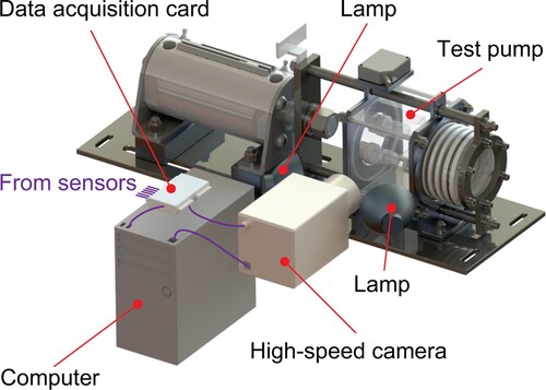
Figure 4. Schematic of the computational domain.

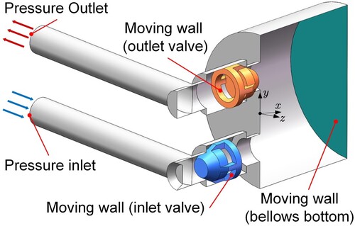
Figure 5. Structured mesh used for the simulation. Different domains are illustrated with different colours. Enlarged views show local refinements in the near-wall region and the region around the end-ring of the inlet valve.

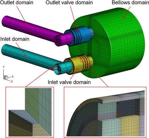
Figure 6. Distribution of time-averaged $y^{+}$ during the suction stroke (Case 1).

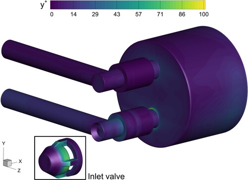
Table 4. Estimations of discretization error.

Parameter	$\varphi =\overline{Q}$
$N_1$,$N_2$,$N_3$	1,259,640, 561,736, 237,408
$r_{21}$,$r_{32}$	1.31, 1.33
${\varphi }_1$,${\varphi }_2$,${\varphi }_3$	13.55, 13.47, 13.35
p	1.63
${\varphi }_{ext}^{21}$,${\varphi }_{ext}^{32}$	13.68, 13.67
$e_a^{21}$,$e_a^{32}$	0.55%, 0.93%
$e_{ext}^{21}$,$e_{ext}^{32}$	0.99%, 1.4%
$GC{I}_{21}$,$GC{I}_{32}$	1.25%, 1.95%

Table 5. Information of meshes used for grid independence analysis.

Mesh	Number of elements	Approx. computational time ($\mathrm{h}$)	ε
Coarse	237,408	37	4.65%
Medium	561,736	56	3.76%
Fine	1,259,640	84	3.22%

Figure 7. Schematic of the forces acting on the inlet check valve at the opening process and details of layering technique for mesh reconstruction.

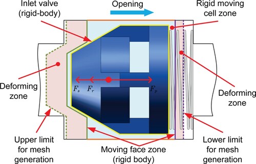
Table 6. Summary of the settings of the fluid solver.

Settings	Details
Pressure-velocity coupling	PISO
Turbulence model	SST $k-\omega$
Multiphase model	Mixture
Cavitation model	Schnerr–Sauer
Spatial discretization	Pressure	PRESTO!
	Momentum	Second-order upwind
	Turbulent kinetic energy	First-order upwind
	Turbulent dissipation rate	First-order upwind
	Volume fraction	First-order upwind
Transient formulation	First-order implicit
Under-relaxation factors	Pressure	0.3
	Momentum	0.7
	Turbulent kinetic energy	0.8
	Turbulent dissipation rate	0.8
	Volume fraction	0.5
Residuals	Continuity	${10}^{-3}$
	X-velocity	${10}^{-5}$
	Y-velocity	${10}^{-5}$
	Z-velocity	${10}^{-5}$
	Turbulent kinetic energy	${10}^{-5}$
	Turbulent dissipation rate	${10}^{-5}$
	Volume fraction	${10}^{-5}$
Time step size $\left(\mathrm{s}\right)$	$2.5\times {10}^{-5}$
Max iteration per time step	50

Figure 8. Comparison of time-averaged flow rate $\overline{Q}$ computed by numerical model and that obtained from experimental measurement at different inlet pressure $p_{\mathrm{i}\mathrm{n}}$. The bottom figure shows the error ϵ between the numerical results and the fitted values of the experimental results.

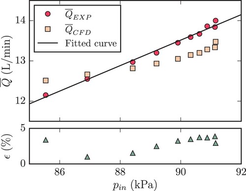
Figure 9. High-speed captures of typical vapour structures in PDBPs (Case 1). (a) Sheet-like cavities at the corner (intersection of the inlet pipe and the inlet channel). (b) Ribbon-like cavities at the core of the inlet channel. (c) Cavitation at the bottom of the inlet valve.

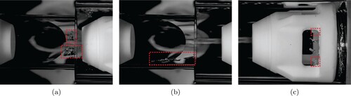
Figure 10. Initiation and development process of vapour structures (iso-surfaces of ${\alpha }_v=0.01$ coloured by blue, ${\alpha }_v=0.5$ coloured by red) at the bottom of the inlet valve when it is fully opened (Case 1). $T_0$ is the instant when cavitation incepts at the bottom of the inlet valve. (a) $T_0$. (b) $T_0+0.2\mathrm{m}\mathrm{s}$. (c) $T_0+0.4\mathrm{m}\mathrm{s}$. (d) $T_0+0.6\mathrm{m}\mathrm{s}$. (e) $T_0+0.8\mathrm{m}\mathrm{s}$ and (f) $T_0+1.0\mathrm{m}\mathrm{s}$.

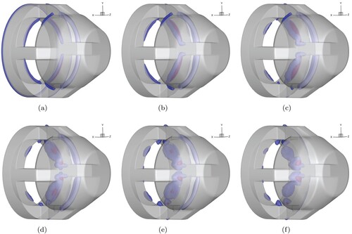
Figure 11. Typical evolution process of vapour structures at the bottom of the inlet valve captured by high-speed camera (Case 1). The vapour structures near the guide bar at the inner part of the end-ring are outlined by red dashed curves. The shed vapour filaments are indicated by orange dashed circles. The time interval between the two frames is $0.5\mathrm{m}\mathrm{s}$.

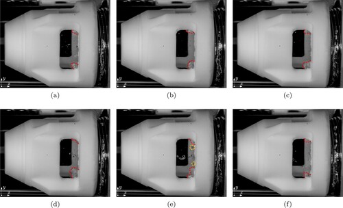
Figure 12. Time series of volume-averaged shear rate $\mathcal{S}$ in different parts of PDBPs from the beginning of the suction stroke (Case 1).

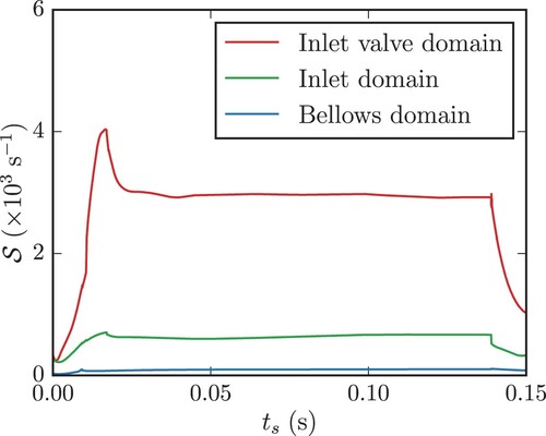
Figure 13. Histograms of time-averaged shear rate $\overline{S}$ in the inlet valve case during the suction stroke (Case 1).

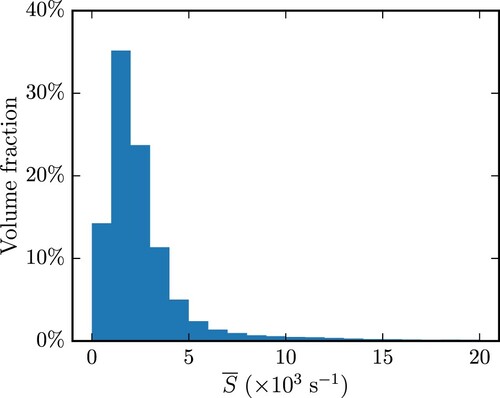
Figure 14. Contour of time-averaged shear rate $\overline{S}$ at different slices of the inlet valve during the suction stroke (Case 1).

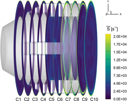
Figure 15. Evolution process of vortical structures (iso-surfaces of $\mathrm{\Omega }=0.52$ coloured by green) at the bottom of the inlet valve when it is fully opened (Case 1). $T_0$ is the instant when cavitation incepts at the leading edge of the end-ring. (a) $T_0$. (b) $T_0+0.2\mathrm{m}\mathrm{s}$. (c) $T_0+0.4\mathrm{m}\mathrm{s}$. (d) $T_0+0.6\mathrm{m}\mathrm{s}$. (e) $T_0+0.8\mathrm{m}\mathrm{s}$ and (f) $T_0+1.0\mathrm{m}\mathrm{s}$.

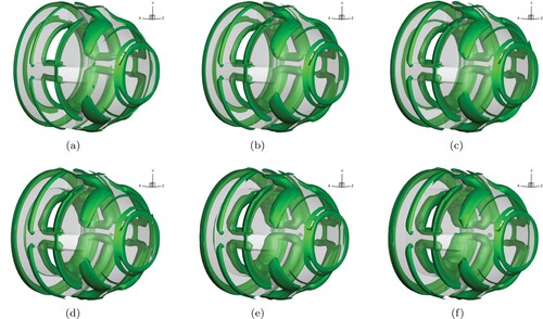
Figure 16. Evolution of the distribution of shear rate S at a cylindrical slice of the inlet valve case, which cuts through the cavities and the vortices at $r\approx 0.47d$ (Case 1). $T_0$ is the instant when cavitation incepts at the leading edge of the end-ring. A cylindrical coordinate system is established to facilitate the analysis. (a) $T_0$. (b) $T_0+0.2\mathrm{m}\mathrm{s}$. (c) $T_0+0.4\mathrm{m}\mathrm{s}$. (d) $T_0+0.6\mathrm{m}\mathrm{s}$. (e) $T_0+0.8\mathrm{m}\mathrm{s}$ and (f) $T_0+1.0\mathrm{m}\mathrm{s}$.

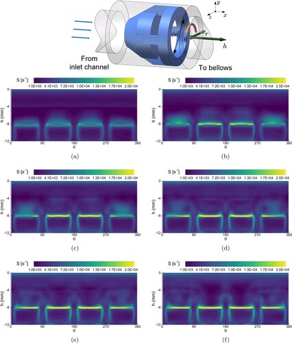
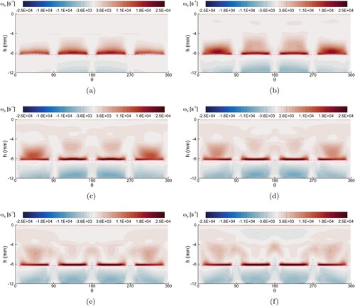
Figure 17. Evolution of the distribution of circumferential vorticity ${\omega }_{\theta }$ at a cylindrical slice of the inlet valve case, which cuts through the cavities and the vortices at $r\approx 0.47d$ (Case 1). $T_0$ is the instant when cavitation incepts at the leading edge of the end-ring. (a) $T_0$. (b) $T_0+0.2\mathrm{m}\mathrm{s}$. (c) $T_0+0.4\mathrm{m}\mathrm{s}$. (d) $T_0+0.6\mathrm{m}\mathrm{s}$. (e) $T_0+0.8\mathrm{m}\mathrm{s}$ and (f) $T_0+1.0\mathrm{m}\mathrm{s}$.