An efficient implementation of compact third-order implicit reconstruction solver with a simple WBAP limiter for compressible flows on unstructured meshes

Figures & data

Figure 1. The compact stencils for interior cell (left) and boundary cell (right).

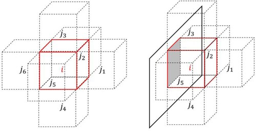
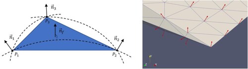
Figure 2. A curved triangle boundary face (left) and vertex normal vectors around sharp geometry (right).

Table

Algorithm 1. Curved wall boundary reconstruction.
For $f=1,2,\dots ,nBoundaryFaces$ do
For $p=1,2,\dots ,nFaceVertices$ do
For $s=1,2,\dots ,nVertexFaces$ do
If $\mathit{S}{\mathit{f}}_s\cdot \mathit{S}{\mathit{f}}_f>0$ then
$\mathit{S}{\mathit{f}}_p+=\mathit{S}{\mathit{f}}_s,\left|\mathit{S}{\mathit{f}}_p\right|+=\left|\mathit{S}{\mathit{f}}_s\right|$
End if
${\mathit{n}}_p=\mathit{S}{\mathit{f}}_p/\left|\mathit{S}{\mathit{f}}_p\right|$
End for
Add $F\left({\xi }_p,{\eta }_p,0\right)=0,[F_x,F_y,F_z{]}_p=\frac{{\mathit{n}}_p}{{\mathit{n}}_p\cdot {\mathit{n}}_f}$ to linear equations
End for
Compute coefficients of $F\left(\xi ,\eta ,h\right)=0$ by solving linear equations
End for

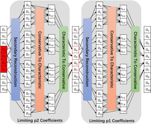
Figure 3. Troubled cells marked by red in limiting procedure.

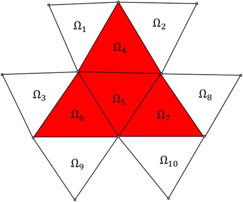
Figure 4. Original WBAP successive limiting procedure.

Table

Algorithm 2. Original WBAP successive limiting procedure.
For $k=p,p-1,\dots ,1$ do
For $i=1,2,\dots ,\text{nCells}$ do
If $I{S}_i>{\overline{S}}_{dis}$ then
For $j=j_1,j_2,\dots ,j_{N_j}$ do
${\hat{U}}_{i,j}^k=R\left({\overline{U}}_i,{\mathit{n}}_{ij}\right)\cdot L\left(R^{-1}\left({\overline{U}}_i,{\mathit{n}}_{ij}\right)\cdot \left(U_i^k,U_{j_1\to i}^k,U_{j_2\to i}^k,\dots ,U_{j_{N_j}\to i}^k\right)\right)$
End for
${\tilde{U}}_i^k=L\left({\hat{U}}_{i,j_1}^k,{\hat{U}}_{i,j_2}^k,\dots ,{\hat{U}}_{i,j_{N_j}}^k\right)$
End if
End for
For $i=1,2,\dots ,\text{nCells}$ do
If $I{S}_i>{\overline{S}}_{dis}$ then
$U_i^k={\tilde{U}}_i^k$
End if
End for
End for

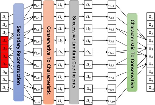
Figure 5. Simple WBAP successive limiting procedure.

Table

Algorithm 3. Simple WBAP successive limiting procedure.
For $f=1,2,\dots ,nFaces$ do
If $\text{max}\left(I{S}_i,I{S}_j\right)>{\overline{S}}_{dis}$ then
$i$ is the left cell of $f$, and $j$ is the right cell of $f$
$\left(V_i,V_j\right)=R^{-1}\left({\overline{U}}_{ij},{\mathit{n}}_{ij}\right)\cdot \left(U_i,U_j\right)$
For $k=p,p-1,\dots ,1$ do
${\hat{V}}_i^k=L\left(V_i^k,V_{j\to i}^k\right),{\hat{V}}_j^k=L\left(V_j^k,V_{i\to j}^k\right)$
$V_i^k={\hat{V}}_i^k,V_j^k={\hat{V}}_j^k$
End for
${\hat{U}}_{i,j}=R\left({\overline{U}}_{ij},{\mathit{n}}_{ij}\right)\cdot V_i,{\hat{U}}_{j,i}=R\left({\overline{U}}_{ij},{\mathit{n}}_{ij}\right)\cdot V_j$
End if
End for
For $i=1,2,\dots ,\text{nCells}$ do
If $I{S}_i>{\overline{S}}_{dis}$ then
${\tilde{U}}_i=L\left({\hat{U}}_{i,j1},{\hat{U}}_{i,j2},\dots ,{\hat{U}}_{i,j{N}_j}\right)$
End if
End for

Table 1. Information of solvers for numerical tests.

Solver	$blastFoam$	$ROUNDA$	$VR3$
Time scheme	RK3SSP	RK3SSP	SDIRK3 GMRES + LUSGS
Grad scheme	Gauss linear	Gauss linear	VR quadratic
Interpolation scheme	Linear vanAlbada	Non-linear low dissipative ROUND	Quadratic polynomial with WBAP limiters
Mesh	Unstructured	Uniform structured	Unstructured

Figure 6. The accuracy test for the schemes of the blastFoam, ROUNDA and VR3.

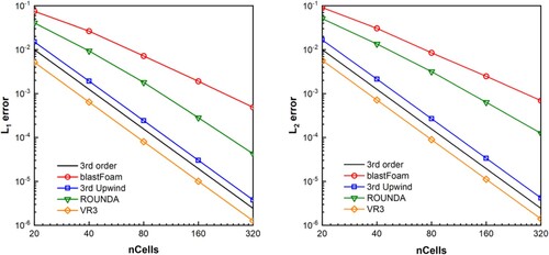
Figure 7. The spectral properties of the schemes of the blastFoam, ROUNDA and VR3.

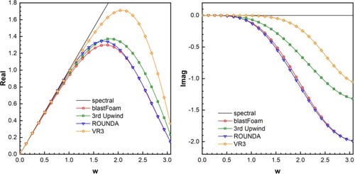
Figure 8. Four successively refined hexahedral meshes for subsonic flow past a sphere.

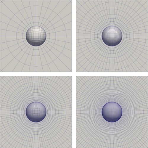
Figure 9. Subsonic flow past a sphere. Computed 31 equally spaced Mach number contours from 0.019 to 0.589 by the three solvers on 32 × 32 × 96 mesh.

Figure 10. Order of error convergence for subsonic flow past a sphere.

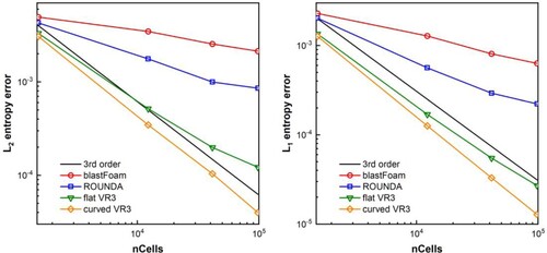
Figure 11. Convergence history comparison for subsonic flow past a sphere with mesh 32 × 32 × 96.

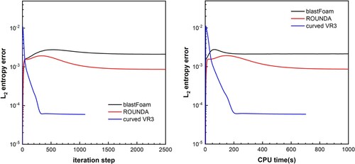
Figure 12. Surface mesh used for transonic flows past a ONERA M6 wing.

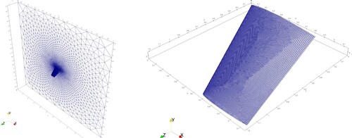
Figure 13. Transonic flows past a ONERA M6 wing. Computed pressure coefficient contours from −1.1 to 1.4.

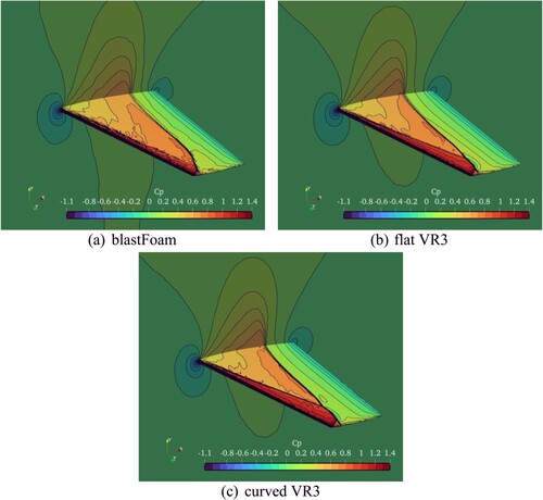
Figure 14. Comparison of experiment and computed surface pressure coefficient of the three methods at different semi-span locations.

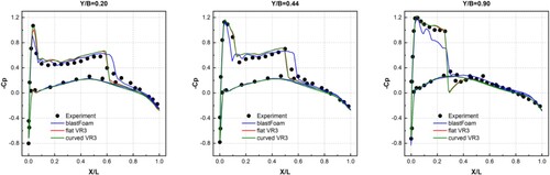
Figure 15. Comparison of entropy production of the three methods at different semi-span locations.

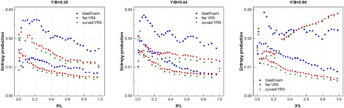
Figure 16. Four types of meshes for isentropic vortex problem.

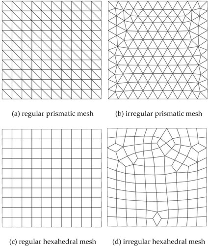
Figure 17. Influence of weights on average inner iteration steps.

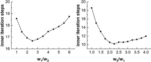
Table 2. Errors and convergence rates for the isentropic vortex problem on four types of meshes.

Mesh type	Size	${\mathit{L}}_1$error	Order	${\mathit{L}}_2$error	Order	${\mathit{L}}_{\mathrm{\infty }}$error	Order
Regular prismatic mesh	$1$	$3.33\text{E}-3$		$7.36\text{E}-3$		$5.91\text{E}-2$
	$1/2$	$2.17\text{E}-4$	$3.94$	$5.24\text{E}-4$	$3.81$	$5.59\text{E}-3$	$3.40$
	1/4	2.61E-5	3.05	$6.36\text{E}-5$	$3.05$	$5.08\text{E}-4$	$3.46$
	$1/8$	2.09E-6	$3.65$	$5.65\text{E}-6$	$3.49$	$6.26\text{E}-5$	$3.02$
Irregular prismatic mesh	$1$	$1.72\text{E}-3$		$3.73\text{E}-3$		$2.49\text{E}-2$
	$1/2$	$2.17\text{E}-4$	$2.99$	$5.24\text{E}-4$	$2.83$	$5.59\text{E}-3$	$2.16$
	$1/4$	1.34E-5	$4.01$	$3.24\text{E}-5$	$4.01$	$2.56\text{E}-4$	$4.45$
	$1/8$	1.35E-6	$3.31$	$4.23\text{E}-6$	$2.94$	$6.42\text{E}-5$	$2.00$
Regular hexahedral mesh	$1$	$9.35\text{E}-3$		$2.22\text{E}-2$		$1.33\text{E}-1$
	$1/2$	$1.39\text{E}-3$	$2.75$	$3.39\text{E}-3$	$2.71$	$2.27\text{E}-2$	$2.55$
	$1/4$	1.55E-4	$3.16$	$3.76\text{E}-4$	$3.17$	$3.53\text{E}-3$	$2.68$
	$1/8$	8.11E-6	$4.26$	$1.98\text{E}-5$	$4.25$	$1.44\text{E}-4$	$4.62$
Irregular hexahedral mesh	$1$			$1.89\text{E}-2$		$1.40\text{E}-1$
	$1/2$	$1.25\text{E}-3$	$2.72$	$2.98\text{E}-3$	$2.67$	$2.32\text{E}-2$	$2.60$
	$1/4$	$1.32\text{E}-4$	$3.25$	$3.19\text{E}-4$	$3.22$	$2.70\text{E}-3$	$3.10$
	$1/8$	$7.02\text{E}-6$	$4.23$	$1.70\text{E}-5$	$4.23$	$1.52\text{E}-4$	$4.15$

Table 3. Comparison of average inner iteration steps of the original weights and the optimized weights in the four types of meshes.

	Original weights	Optimized weights
Regular prismatic mesh	16.925	9.05
Irregular prismatic mesh	20.9	13.025
Regular hexahedral mesh	24.175	16.075
Irregular hexahedr mesh	19.225	21.65

Figure 18. Isentropic vortex evolution after 5 time periods (left) and 10 time periods (right).

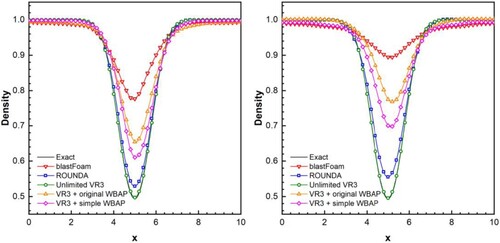
Table 4. Comparison of wall-clock time for different limiters for the smooth isentropic vortex problem on a regular hexahedral mesh at h = 1/8 after 10 time periods.

Limiters	Unlimited	Simple WBAP	Original WBAP
wall-clock time (s)	888	1963	$5189$

Table 5. Two shock tube cases.

Problem	${\rho }_L$	$u_L$	$p_L$	${\rho }_R$	$u_R$	$p_R$	$t_{end}$
Sod	1.0	0.75	1.0	0.125	0.0	0.1	0.2
Lax	0.445	0.698	3.528	0.5	0.0	0.571	0.1

Figure 19. Density distribution of Sod case at t = 0.2 (left) and Lax case at t = 0.1 (right).

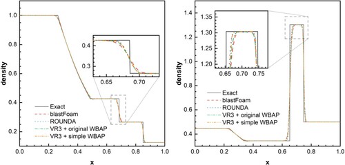
Figure 20. The Shu-Osher problem. Density distribution at t = 1.8.

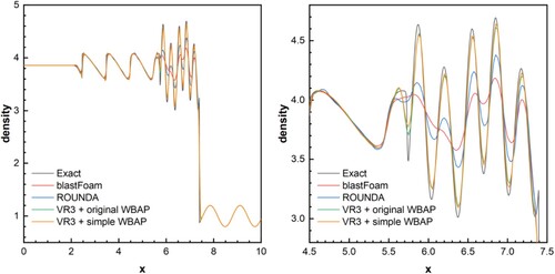
Figure 21. Two blast wave problem. Density distribution at t = 0.038.

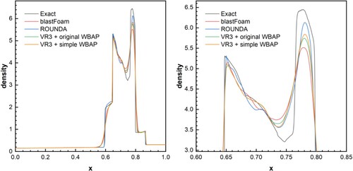
Figure 22. Mach 3 wind tunnel with a step. Thirty equally spaced density contour lines from ρ = 0.3 to 6.15.

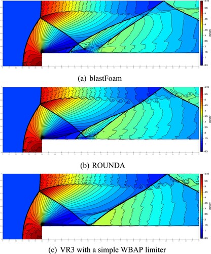
Figure 23. Forward step problem. Troubled cells are marked black.

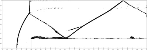
Figure 24. Double Mach reflection. Thirty equally spaced density contour lines from ρ = 1.75 to 21.5.

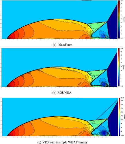
Figure 25. Double Mach reflection problem. Troubled cells are marked black.

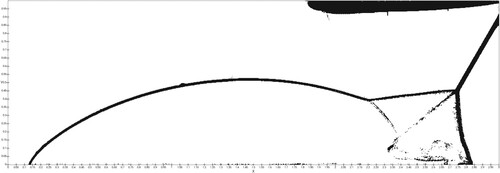
Figure 26. Numerical results for 3D explosion problem in the radial direction at time t = 0.2. Density profile (left) and troubled cells marked (right).

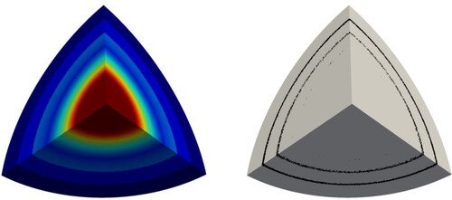
Figure 27. The results distribution along the radius direction.

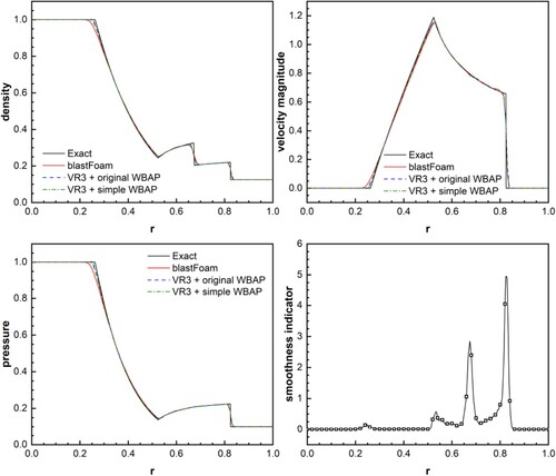
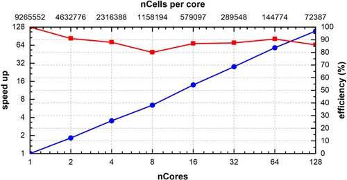
Figure 28. Parallel scaling efficiency of the VR3 solver with a simple WBAP limiter.