Lingual microbiota profiles of patients with geographic tongue

Figures & data

Table 1. Characteristics and sampling of patients with geographic tongue (GT) and healthy age- and sex-matched controls

	Patients with GT (n = 35)	Control (n = 22)
Males (%)	n = 19 (54.3%)	n = 12 (54.5%)
Females (%)	n = 16 (45.7%)	n = 10 (45.5%)
Age (mean ± SD)	54.3 ± 16.1	56.3 ± 15.8
Sampling	n = 69 (n = 34 GT-lesion) (n = 35GT-healthy)	n = 22

SD, standard deviation.

Table 2. Other phyla^a identified among patients with GT and controls

	Number of reads
Phylum	Total	GT-lesion	GT-healthy	Control
Deinococcus-Thermus	3,374	3,286	80	8
Tenericutes	1,198	793	199	206
Acidobacteria	937	832	21	84
Nitrospirae	75	57	18	0
Fibrobacteres	4	0	0	4

^aOther phyla that were demonstrated in Figure 1.

Figure 1. Relative abundance of the bacterial phyla among patients with geographic tongue (GT) and controls. Values shown are means ± standard deviation (SD). Comparisons between the groups were analyzed by the Kruskal–Wallis test; *p < 0.05; ***p < 0.001; ****p < 0.0001. The group ‘other phyla’ comprises the five phyla listed in Table 2.

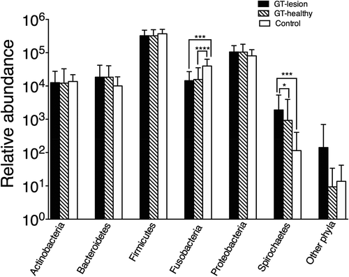
Table 3. Relative abundance of the bacterial taxa that represent >1% of the total reads

		Median (range) % of the relative abundance
Taxon (phylum)	Relative abundance, %^a	Control	GT-lesion	GT-healthy
Streptococcus (Firmicutes)	48.4	4.0 (1.5–12.7)	2.5 (0.2–5.8)	2.7 (0.6–7.1)
Haemophilus (Proteobacteria)	11.1	3.5 (0.6–10.1)	2.3 (<0.1–9.1)	2.1 (0.3–10.7)
Veillonella (Firmicutes)	10.6	3.6 (1.1–12.7)	1.9 (<0.1–11.2)	2.8 (<0.1–6.0)
Neisseria (Proteobacteria)	6.6	2.5 (<0.1–11.4)	1.0 (<0.1–27.7)	1.3 (<0.1–23.3)
Fusobacterium (Fusobacteria)	4.0	4.3 (<0.1–9.9)	1.9 (<0.1–10.2)	1.1 (<0.1–18.4)
Granulicatella (Firmicutes)	2.0	4.1 (0.4–8.5)	2.4 (0.1–12.0)	2.6 (<0.1–8.5)
Gemella (Firmicutes)	1.9	3.9 (0.4–13.3)	1.5 (0.0–9.1)	2.3 (0.1–9.0)
Staphylococcus (Firmicutes)	1.8	0.3 (0.0–45.8)	0.2 (0.0–36.1)	0.04 (0.0–53.6)
Vagococcus (Firmicutes)	1.6	4.6 (0.3–9.6)	2.2 (0.1–9.8)	2.3 (<0.1–9.9)
Prevotella (Bacteroidetes)	1.5	3.1 (0.3–16.8)	1.5 (0.0–32.1)	1.2 (0.0–14.5)
Flavobacterium (Bacteroidetes)	1.5	0.5 (0.0–61.2)	0.4 (0.0–22.8)	0.1 (0.0–37.5)
Actinomyces (Actinobacteria)	1.4	4.8 (0.3–10.6)	1.4 (<0.1–17.2)	1.9 (<0.1–14.2)
Enterococcus (Firmicutes)	1.2	3.0 (0.2–24.2)	1.9 (0.1–18.8)	1.8 (0.0–22.8)

^aRelative abundance for each taxon was calculated as number of reads for the taxon divided with the total number of all the reads across all the samples.

Figure 2. Richness of the lingual microbiota in patients with GT and controls. Bacterial DNA was extracted and the 16S rRNA genes were sequenced and assigned to operational taxonomic units (OTUs) with a minimum pairwise identity of 97.0%. Each symbol represents one individual. Values shown are means ± SD. Comparisons between the groups were analyzed by one-way analysis of variance (ANOVA), **p < 0.01, and a paired t-test ^§§p < 0.01.

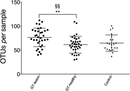
Figure 3. Diversity indexes at the OTU level. (a) Shannon’s index values; (b) Simpson’s index values. Comparisons between the groups were analyzed by one-way ANOVA, ***p < 0.001 (comparisons between all groups), and Wilcoxon’s signed-rank test, ^§§§p < 0.001 (comparisons between the paired samples). The 25th and 75th percentiles are shown in the box plot. The median is indicated by the horizontal solid lines. The bars indicate the minimum to maximum values.

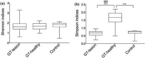
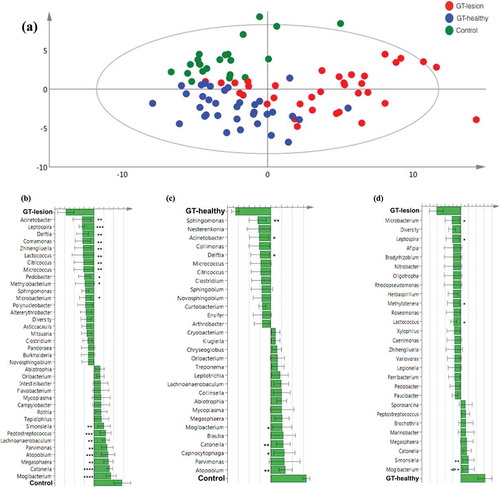
Figure 4. Differences in the lingual microbiota compositions of patients with GT and controls. The presence or absence of 403 identified OTUs was checked in each individual of the three groups. (a) Principal component analysis. Each symbol represents one individual. The 2D illustration shows that subjects that belong to the same group tend to cluster together, whereas those that belong to different groups remain separated from one another. (b–d) Orthogonal partial least square analysis loading plots. Shown are those OTUs that contribute most to distinguishing between the GT-lesion group and the control group (b), the GT-healthy group and the control group (c), and the GT-lesion group and the GT-healthy group (d). OTUs that show the strongest contribution to the respective models were tested for differences in prevalence using Fisher’s exact tests (or paired t-tests for paired samples). *p < 0.05; **p < 0.01; ***p < 0.001; and ^§p < 0.05 for paired t-test.