
Figures & data
Figure 1. Picture on the left (a): the reference points and lines were marked, a and b indicates the smallest width of the posterior and anterior ramus respectively, c indicates the longest length of the planned anterior ramus graft. Picture in the middle (b): Mp is the width of the ramus bone at the mid-point of Sn-An Line. Picture on the right (c): the cross-sectional area of Eo-Md was marked red (x). The tallest and widest part of the cross section were also measured as h and w, respectively.
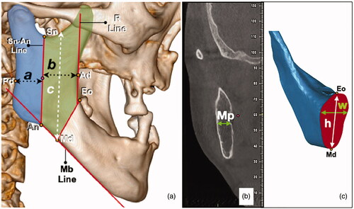
Table 1. Reference points and lines.
Figure 2. Top picture (a): design of osteotomy; bottom picture (b): rotation of graft. The grey area shows the pathological defect marked with reference to the CT scans. The yellow area indicates the anterior ramus graft. The blue area indicates the remnant coronoid process after the osteotomy. The green lines are the reference lines (Mb Line and R Line). The black dotted lines are the designed osteotomy lines. The black arrows indicate area of deficiency which can be filled by the remnant coronoid process.
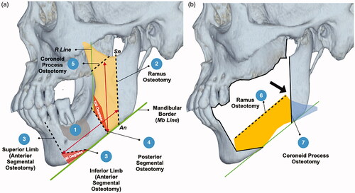
Table 2. Clinical application.
Figure 3. The upper left picture (a) shows the 3D simulation of the unoperated mandible. Pictures (b–d) demonstrates the rotation of the graft. Gray – area to be resected; yellow – anterior ramus graft; blue – remnant coronoid bone; pink – remaining native bone. The red arrow points to the pathological defect.
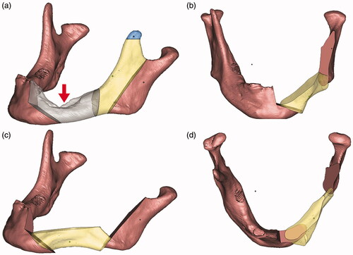
Figure 4. Picture on the upper left corner (a), fitting of the surgical guides; (b) pre-bending of reconstruction plate according to the contour of the 3D printed pre-operative mandible; (c) the 3D printed mandible was cut according to the guides; (d) temporary fixation of the reconstruction plate to the mandible; (e and f) fitting of the anterior ramus graft.
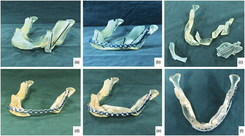
Figure 5. (a) Osteotomy lines; (b) the mandibular segmental defect; (c and d) superior and inferior view of reconstructed mandible; (e) Resected pathology; (f) the red dashed line demonstrate the natural curvature of the anterior border of the ramus – upon rotation, this will form inferior border of the reconstructed mandible. The internal oblique ridge is marked within a green dashed circle.
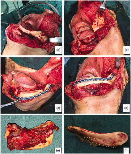
Figure 6. Pre-operative and post-operative computed tomographies (3D reconstructed).
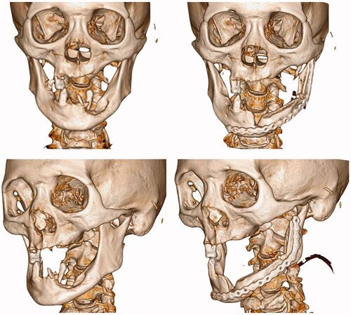
Figure 7. Intra-oral and extra-oral photographs (taken after 12 months post-operatively).
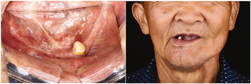
Figure 8. Comparison between the postoperative computed tomographies taken after 1 month and 12 months respectively. Note the radiopaque bone bridge between the grafted bone and the native bone.
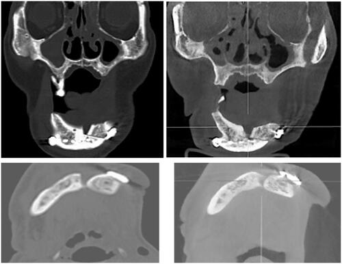
Figure 9. Bone scan taken 12 months post-operatively indicates the viability of the grafted bone.
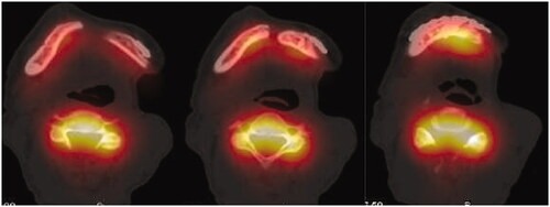
Figure 10. Representative images of another case. The picture on the left shows the intra-operative clinical photos while the picture on right shows the post-operative CT Scan.
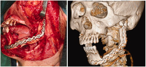
Table 3. Proposed criteria for case selection.