Figures & data
Figure 1. Schematic of the exosome isolation protocol from solid brain tissue. Fresh frozen (−80°C) human frontal cortex was sliced with a razor blade on ice while frozen to generate 1–2 cm long, 2–3 mm wide sections. The cut sections are dissociated while partially frozen in 75 U/ml of collagenase type 3 in Hibernate-E at 37°C for a total of 20 min. The tissue is returned to ice immediately after incubation and protease and phosphatase inhibitors are added. The tissue is spun at 300 × g for 5 min at 4°C (pellet is used as the brain homogenate + collagenase control), the supernatant transferred to a fresh tube, spun at 2000 × g for 10 min at 4°C, then at 10,000 × g for 30 min at 4°C. The EV-containing supernatant is overlaid on a triple sucrose cushion (0.6 M, 1.3 M, 2.5 M) and ultracentrifuged for 3 h at 180,000 × g to separate vesicles based on density. The top of the gradient is discarded and fractions designated 1, 2 and 3 are collected and the refractive index is measured. Each fraction is further ultracentrifuged at 100,000 × g to pellet the vesicles contained in each fraction. Each preparation is validated by a combination of techniques including electron microscopy and RNA and protein analysis. Note – some tissue samples will not be amenable to this method. Post-mortem delay, storage time and the number of freeze-thaw cycles will negatively impact on tissue quality and result in contamination of the fractions with cellular debris and non-exosome vesicles.
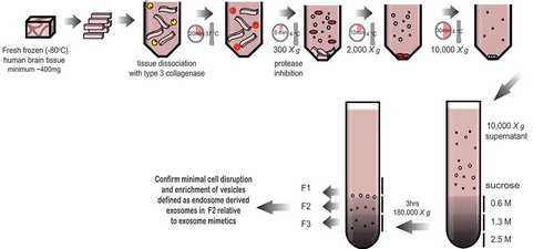
Figure 2. Transmission electron microscopy (a + b) and dynamic light scattering (b + c) of frontal cortex vesicles. Vesicle fractions 1–3 were visualized by negative-staining transmission electron microscopy: (a) scale bar represents 500 nm or (b) 200 nm. TEM is representative of 5 images taken of each fraction from 30 independent human tissue samples. To further corroborate the diameter of the vesicles, fractions were subject to dynamic light scattering to determine the relative size distribution. DLS signal intensity (c) was transformed to percentage volume distribution (d). The thin black line represents F1, thick black like F2 and thick grey line F3. The analysis was performed in size mode with all measurements made in triplicate. An average of three independent tissue samples is shown.
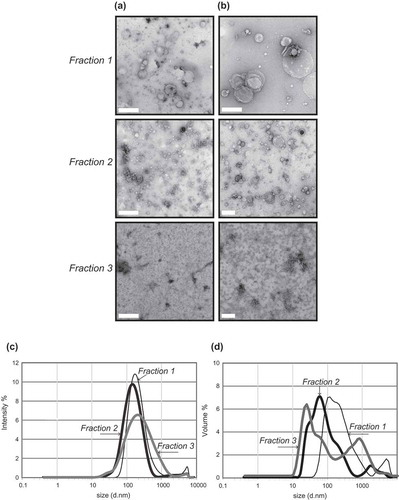
Figure 3. Western blot analysis of frontal cortex and associated vesicles. Equivalent protein from human frontal cortex brain homogenate without (BH) and with collagenase (BH + C) and three vesicle fractions were separated by gel electrophoresis and the total protein load was visualized using stain-free technology or ponceau S membrane staining. Immunoblotting was carried out using antibodies to BiP, calnexin, calreticulin, VDAC,, flotillin-1, syntenin, TSG101 and CD81. Immunoblots are representative of at least five independent experiments.
Figure 4. Proteomic analysis of frontal cortex vesicles. Proteins extracted from vesicle fractions 1–3 were submitted to proteomic analysis. A three-way Venn diagram of proteins (minimum two peptides detected) distributed between three independent biological replicates is shown. An average of 978 proteins were identified in F1 with 571 proteins common across the biological replicates, an average of 1567 proteins identified in F2 with 1144 common proteins and an average of 1300 proteins identified in F3 with 815 common proteins. Some exosomal proteins unique to F2 are listed. Venn diagrams were generated using the FunRich open-access tool Citation[20].
![Figure 4. Proteomic analysis of frontal cortex vesicles. Proteins extracted from vesicle fractions 1–3 were submitted to proteomic analysis. A three-way Venn diagram of proteins (minimum two peptides detected) distributed between three independent biological replicates is shown. An average of 978 proteins were identified in F1 with 571 proteins common across the biological replicates, an average of 1567 proteins identified in F2 with 1144 common proteins and an average of 1300 proteins identified in F3 with 815 common proteins. Some exosomal proteins unique to F2 are listed. Venn diagrams were generated using the FunRich open-access tool Citation[20].](/cms/asset/9906cb3b-4aed-4935-bc04-0d0021ea4707/zjev_a_1348885_f0004_oc.jpg)
Figure 5. Analysis of cellular component GO terms. The proteins common to each fraction were grouped using gene ontology (GO) terms related to cellular component analysis process using DAVID Citation[19]. The graph shows the percentage of proteins identified by mass spectrometry that fall into the designated GO category relative to the total number of proteins in the category. GO FAT was used to minimize the redundancy of general GO terms in the analysis. A modified Fisher’s exact p-value was used to demonstrate gene ontology, where p-values less than 0.05 after Benjamini multiple test correction were considered enriched in the category. A count threshold of 5 and default value of 0.05 for the enrichment score was used. Categories with enrichment greater than 5.5% are shown.
![Figure 5. Analysis of cellular component GO terms. The proteins common to each fraction were grouped using gene ontology (GO) terms related to cellular component analysis process using DAVID Citation[19]. The graph shows the percentage of proteins identified by mass spectrometry that fall into the designated GO category relative to the total number of proteins in the category. GO FAT was used to minimize the redundancy of general GO terms in the analysis. A modified Fisher’s exact p-value was used to demonstrate gene ontology, where p-values less than 0.05 after Benjamini multiple test correction were considered enriched in the category. A count threshold of 5 and default value of 0.05 for the enrichment score was used. Categories with enrichment greater than 5.5% are shown.](/cms/asset/cfefffc1-3534-4c65-9fab-e5d032872a1c/zjev_a_1348885_f0005_oc.jpg)
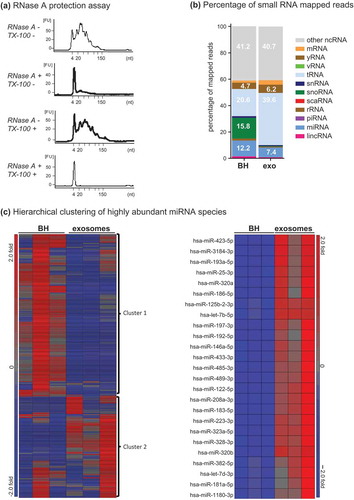
Figure 6. Small RNA analysis of Fraction 2. (a) Bioanalyser analysis of small RNA associated with Fraction 2. Fraction 2 was treated with or without Triton-X 100 and or RNase A for 30 min, RNA was extracted and analysed on a small RNA chip which was submitted for bioanalysis. miRNA is between 4 and 22 nt in length. The peak visualized at 4 nt is the marker peak. (b + c) Analysis of RNase A-treated small RNA. Raw sequencing reads were aligned to the human genome (HG19) and mapped to miRBase V.20 and other small RNA from Ensembl Release 17 followed by normalization of raw reads to reads per million (RPM). The mean of reads per miRNA (n = 3) was calculated. (b) The percentage of total reads mapped to non-coding small RNA and other RNA species identified by small RNA deep sequencing. (c) Left panel, unsupervised hierarchical clustering of highly abundant miRNA species (>10 RPM) identified in BH and F2 (n = 3, all groups). Cluster 1 miRNAs are enriched in BH and cluster 2 miRNAs are enriched in F2. Right panel, unsupervised hierarchical clustering of the top 20 miRNA detected in F2. Red indicates high expression and blue indicates low expression.