Figures & data
Figure 1. Schematic of the TIGER sRNA-seq analysis workflow. Total reads from sRNA-seq platform are filtered through pre-processing steps (green) to yield total quality reads. Filtered reads are then applied to a class-independent analysis (red), which compares the most abundant reads of each sample/group, regardless of mapping identity. Independently, filtered reads are aligned to the host genome (e.g. mouse; light blue) and categorized by sRNA type for analysis. Quality reads that are >19 nt that failed to align to the host genome are then separately aligned to either bacterial and fungal genome databases (purple) or exogenous rRNA, RNA and miRNA databases (gold). Results of host and non-host segments of the pipeline are summarized and plotted (navy). Lastly, reads that fail to map in host and non-host segments are sorted by abundance for comparison and submitted for BLASTn to identify putative origins (orange).
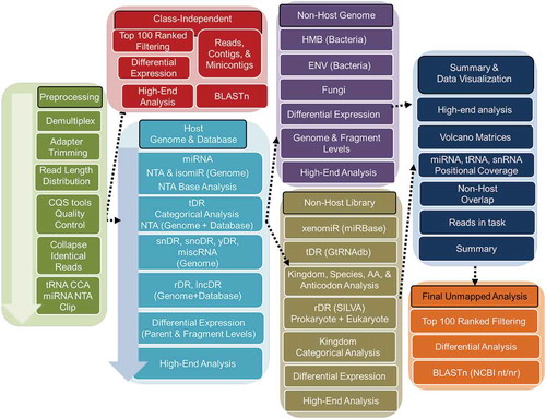
Figure 2. Endogenous miRNA profiles are unique among lipoproteins, biofluids and tissue. WT: wild-type mice; SR-BI KO: Scavenger receptor BI Knockout mice (Scarb1−/-). (a) Correlation of sRNA-seq reads per million total reads (RPM, blue) and miRNA reads (RPM miR, grey) to real-time PCR relative quantitative values (RQV). Spearman correlation. HDL, APOB, liver, bile and urine samples, N = 66. (b-f) Results from sRNA-seq analysis of murine miRNA. HDL WT, N = 7; HDL SR-BI KO N = 7; APOB WT, N = 7, APOB SR-BI KO N = 7; Liver WT, N = 7; Liver SR-BI KO, N = 7; Bile WT, N = 7; Bile SR-BI KO, N = 6; Urine WT, N = 5; Urine SR-BI KO, N = 6. (b) Summary of total miRNA counts per million total (quality) sequencing reads. Mean ± S.E.M. (c) Principal Coordinate Analysis (PCoA) of canonical miRNA profiles for samples from WT (empty circles) and SR-BI KO (filled circles) mice. NMDS1: Non-metric multidimensional scaling. (d) Heatmap of hierarchical clustered pairwise correlation coefficients (Spearman, R) between group means for canonical miRNAs. (e) Start position analysis of 5ʹ miRNA variants (isomiR) for combined (WT and SR-BI KO) mouse samples. (f) Ratio of non-templated U (uridylation) to A (adenylation) for miRNAs. Mean ± S.E.M. One-way ANOVA. *p < 0.05; **p < 0.01.
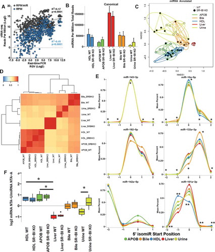
Figure 3. The non-miRNA, host sRNAs landscape distinguishes lipoproteins, biofluids and tissue. WT: wild-type mice; SR-BI KO: Scavenger receptor BI Knockout mice (Scarb1−/-). (a–f) Results from sRNA-seq analysis. HDL WT, N = 7; HDL SR-BI KO N = 7; APOB WT, N = 7, APOB SR-BI KO N = 7; Liver WT, N = 7; Liver SR-BI KO, N = 7; Bile WT, N = 7; Bile SR-BI KO, N = 6; Urine WT, N = 5; Urine SR-BI KO, N = 6. Host tDRs (yellow), rDRs (red), miRNAs (blue), snoDRs (purple), snDRs (green), other small (os)RNA (pink) and unannotated genome (black). (a) Alignment summary of endogenous sRNA classes relative to total reads. Mean ± S.E.M. (b-f) Distribution of read lengths for host sRNA classes (colours) displayed upon the distribution of total reads (grey), as reported by reads per million total reads. Mean ± S.E.M. (b) Liver. (c) APOB. (d) HDL. (e) Bile. (f) Urine.
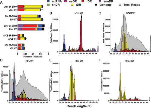
Figure 4. Fragment analysis of tRNA-derived sRNAs provides resolution between sample types with similar tRNA composition. WT: wild-type mice; SR-BI KO: Scavenger receptor BI Knockout mice (Scarb1−/-). (a–c, f) Results from sRNA-seq analysis. (a) Positional coverage maps of tDRs for parent tRNA amino acid anti-codons, as reported as mean cumulative read fractions (read counts/total counts). (b–c) Principal Coordinate Analysis (PCoA) of tDR profiles based on (b) parent tRNAs and (c) individual tDR fragments for samples from WT (white circles) and SR-BI KO (black circles) mice. NMDS: non-metric multidimensional scaling. (d–f) Real-time PCR analysis of candidate tDRs with predicted folding structures and sequences for (d) tDR-GluCTC and (e) tDR-GlyGCC. WT: white circles; SR-BI KO: red circles. Note: Buffer sample corresponds with total RNA extracted from SEC buffer used to isolate lipoproteins. (f) Heatmaps of correlation coefficients (Spearman, R) for tRNA parents and individual tDR fragments across samples within each group. HDL WT, N = 7; HDL SR-BI KO N = 7; APOB WT, N = 7, APOB SR-BI KO N = 7; Liver WT, N = 7; Liver SR-BI KO, N = 7; Bile WT, N = 7; Bile SR-BI KO, N = 6; Urine WT, N = 5; Urine SR-BI KO, N = 6.
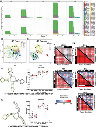
Figure 5. Lipoproteins are enriched for exogenous non-host tDRs and rDRs. WT: wild-type mice; SR-BI KO: Scavenger receptor BI Knockout mice (Scarb1−/-). (a) Stacked bar plots of non-host tDRs aligned to parent tRNAs across kingdoms and higher organizations – bacteria, blue; eukaryota, yellow; fungi, red; embryophyta, orange; vertebrata, purple; archaea, green – as reported as reads per million total reads. (b) Positional coverage maps of non-host tDRs for parent tRNA amino acid anti-codons, as reported as mean cumulative read fractions (read counts/total counts) for HDL and APOB particles. (c) Stacked bar plots of non-host rDRs aligned to parent rRNAs across kingdoms and higher organizations – bacteria, yellow; eukaryota, red; fungi, white; protists, purple; archaeplastida, dark blue; embryophyta, light blue; archaea, green – as reported as reads per million total reads. (d–e) Distribution of read lengths, as reported reads per million total reads, for all non-host (d) tDRs and (e) rDRs. Two-tailed Student’s t-tests. *p < 0.05. HDL WT, N = 7; HDL SR-BI KO N = 7; APOB WT, N = 7, APOB SR-BI KO N = 7; Liver WT, N = 7; Liver SR-BI KO, N = 7; Bile WT, N = 7; Bile SR-BI KO, N = 6; Urine WT, N = 5; Urine SR-BI KO, N = 6.
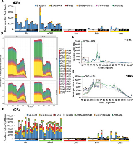
Figure 6. Exogenous sRNAs on lipoproteins are predominantly derived from Proteobacteria in the microbiome and environment. WT: wild-type mice; SR-BI KO: Scavenger receptor BI Knockout mice (Scarb1−/-). (a) Circular tree maps for non-host bacterial sRNAs on HDL from WT mice, as organized by taxonomy. Diameter is proportional to the mean number of reads at the genome level (counts). (b–c) Heatmaps of correlation coefficients (Spearman, R) for non-host sRNAs (on HDL and APOB particles) for bacterial genomes and individual bacterial fragments across samples grouped by (b) human microbiome (HMB) and (c) environment (ENV) species. (d–e) Distribution of read lengths, as reported as percent of total reads, for non-host bacterial sRNAs grouped by (d) HMB and (e) ENV species. Two-tailed Student’s t-tests. *p < 0.05. (f–g) Real-time PCR analysis of candidate non-host bacterial sRNAs for (f) exogenous rDR Pseudomonas fluorescens 23S (exo_rDR_Pflo23S) and (g) exogenous rDR Janthinobacterium lividum 23S (exo_rDR_Jliv). Note: Buffer sample corresponds with total RNA extracted from SEC buffer used to isolate lipoproteins. WT: white circles; SR-BI KO: red circles. HDL WT, N = 7; HDL SR-BI KO N = 7; APOB WT, N = 7, APOB SR-BI KO N = 7; Liver WT, N = 7; Liver SR-BI KO, N = 7; Bile WT, N = 7; Bile SR-BI KO, N = 6; Urine WT, N = 5; Urine SR-BI KO, N = 6.
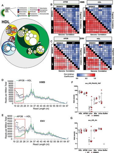
Figure 7. Class-independent analysis defines sRNA content across lipoproteins, biofluids and tissues. (a–e) Circos plots linking the most abundant (top 100) sequences to assigned groups for non-host libraries (rRNA lib, tRNA lib), host sRNAs (rDR, osRNA, tDRs, snDRs, snoDRs and miRNAs) and non-host genomes (fungi, environment, and microbiome) for (a) liver, (b) bile, (c) APOB, (d) HDL and (e) urine. (f) Principal Coordinate Analysis (PCoA) of sRNA profiles based on class-independent analyses. Wild-type mice, WT (open circles); Scavenger receptor BI Knockout mice (Scarb1−/-), SR-BI KO (filled circles). HDL WT, N = 7; HDL SR-BI KO N = 7; APOB WT, N = 7, APOB SR-BI KO N = 7; Liver WT, N = 7; Liver SR-BI KO, N = 7; Bile WT, N = 7; Bile SR-BI KO, N = 6; Urine WT, N = 5; Urine SR-BI KO, N = 6.
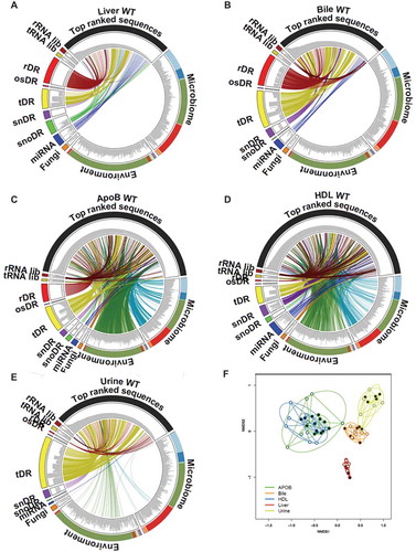
Figure 8. TIGER analysis pipeline identifies more sequencing depth than other software. (a–b) Ternary plots of sRNA profiles for all samples displayed as (a) percent unexplained (blue axis), miRNAs (green axis) and non-miRNA host sRNAs (red axis); (b) percent unexplained (blue axis), exogenous sRNAs (green axis) and host genome (red axis). WT: wild-type mice; SR-BI KO: Scavenger receptor BI Knockout mice (Scarb1−/-). (c) Pie charts illustrating the mean fraction of reads assigned to host sRNA (red), host genome (blue), non-host (purple), too short for exogenous mapping (green) and unmapped (orange). HDL WT, N = 7; HDL SR-BI KO N = 7; APOB WT, N = 7, APOB SR-BI KO N = 7; Liver WT, N = 7; Liver SR-BI KO, N = 7; Bile WT, N = 7; Bile SR-BI KO, N = 6; Urine WT, N = 5; Urine SR-BI KO, N = 6. (d) Comparisons of sRNA-seq data analysis pipelines, as reported as percent assigned per total reads for TIGER (black), Chimira (blue), Oasis (red), ExceRpt (green), and miRge (yellow) for HDL, APOB, and liver samples from WT mice. HDL WT, N = 7; APOB WT, N = 7, Liver WT, N = 7. Mann–Whitney non-parametric tests. *p < 0.05.
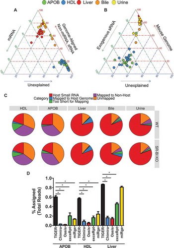
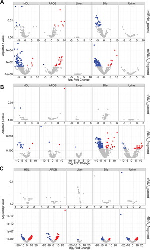
Figure 9. Differential expression analysis at the fragment level identifies differences between SR-BI KO and wild-type mice. Differential expression analysis by DEseq2. Volcano plots demonstrating significant (adjusted p > 0.05) differential (>1.5-absolute fold change) abundances for (a) miRNAs, (b) tDRs and (c) rDRs at the parent and individual fragment levels – red, increased; blue, decreased. HDL WT, N = 7; HDL SR-BI KO N = 7; APOB WT, N = 7, APOB SR-BI KO N = 7; Liver WT, N = 7; Liver SR-BI KO, N = 7; Bile WT, N = 7; Bile SR-BI KO, N = 6; Urine WT, N = 5; Urine SR-BI KO, N = 6.