Figures & data
Figure 1. TEM ExosomeAnalyzer workflow overview.
Usually, TEM images (a) of EVs are manually analysed, which is time consuming. TEM ExosomeAnalyzer is able to detect EVs with almost no input from the user. (b) EVs manually labelled by experts; these images served as the references for the software tool performance being evaluated in three different modes (with decreasing levels of automatic analysis and concurrently with increasing levels of human interaction). The Fully automatic mode (left column – c and c’), Filtered seeds mode (middle column – d and d’) and Curated seeds mode (right column – e and e’). Lime green colour highlights processes performed by the software tool, while magenta colour corresponds to processes performed by the user. In the first step of automatic detection, seeds (= centres) of EVs are found (c) and in the second step EVs are segmented (= their borders are found) (c’). Seeds of EVs which do not meet the requirements set in “Parameters” prior analysis are filtered out in segmentation step. An example is shown in box 2; in detection step, five seeds were found (white arrowheads) (c), but after segmentation (c’), only three EVs remained and two original seeds (dark blue and light green) were filtered out due to their size lower than 30 nm (default value, adjustable). If the user is not satisfied with detected seeds, the seeds at wrong positions can be manually deleted (d), and then segmented (d’), pink and dark green seeds in box 2 serve as an example. Moreover, if some seeds are missing, they can be manually added (e) and then segmented (e’), orange seed in box 1 serves as an example. If the user is not satisfied with segmentation results, they can be also modified prior the export of results. Finally, qualitative (images and masks) and quantitative results including diameter, roundness, perimeter and area of EVs are exported (f).
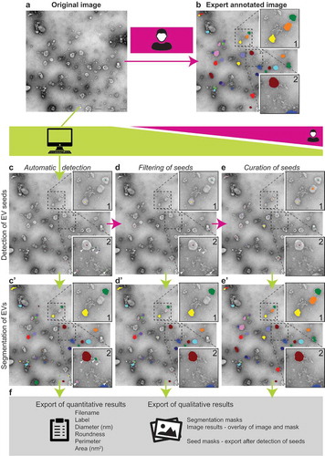
Figure 2. Performance of TEM ExosomeAnalyzer – homogeneous dataset.
The performance of TEM ExosomeAnalyzer was compared with images manually annotated by experts. (a) Four representative images from a small (12 images) homogeneous dataset with all samples prepared and images taken on the same day using identical magnification. The white bar represents 200 nm in each image. (b) Graphs showing performance of the software tool in three categories – Precision (left panel), Recall (middle panel) and F1 score (right panel), each time for three different modes (fully automatic, filtered seeds and curated seeds – as described in ). Each symbol in the graphs corresponds to result for one image. Red colour highlights performance of the software tool for the second image from (a) which was chosen as an example. In Filtered seeds all wrong seeds are removed, therefore all the remaining ones are correct leading to nearly perfect Precision, however, some EVs have still not been detected (no seeds had been added), therefore there is no improvement in terms of number of correctly recognised EVs (Recall), which can be observed as no difference between Fully automatic and Filtered seeds in Recall. (c) The software tool performance depicted as histogram of relative frequencies with respect to diameter of detected EVs. Histograms for manually annotated images and for images analysed by TEM ExosomeAnalyzer are shown together with intersections of manual detection with each of the evaluated modes. (d) Table summarising the results from dataset analysis at the level of individual EVs (not on image levels as in (b)).
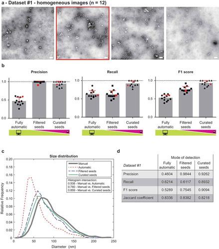
Figure 3. Performance of TEM ExosomeAnalyzer – highly heterogeneous dataset.
TEM ExosomeAnalyzer performance was compared to expert annotated images. (a) shows 18 representative images of highly heterogeneous dataset (30 images altogether) containing images of EVs from multiple sources (patient ascites and several cell cultures), isolated by multiple researchers and visualised by TEM using various magnifications and on different days. The white bar represents 200 nm in each image. (b) Graphs showing performance of the software tool in three categories – Precision, Recall and F1 score, each time for three different modes (fully automatic, filtered seeds and curated seeds – as described in ). Each symbol in the graphs corresponds to result for one image. Similarly as in , in Filtered seeds all wrong seeds are removed, therefore all the remaining ones are correct leading to nearly perfect Precision, however, some EVs have still not been detected (no seeds added), therefore there is no improvement in terms of number of correctly recognised EVs (Recall), which can be observed as no difference between Fully automatic and Filtered seeds in Recall. Five images are highlighted by colour (red, yellow, green, violet and blue) both in (a) and (b) to illustrate the performance of the software tool for individual images with different level of heterogeneity. (c) The software tool performance shown as histogram of relative frequencies with respect to diameter of detected EVs. Histograms for manually annotated images as well as for images analysed by the software tool are shown together with intersections of manual detection with each of the semi-automated analyses. Using the Curated seeds mode, we were able to detect EVs with precision higher than 85 %. (e) Table summarising the results from dataset analysis at the level of individual EVs (not on image levels as in (b)).
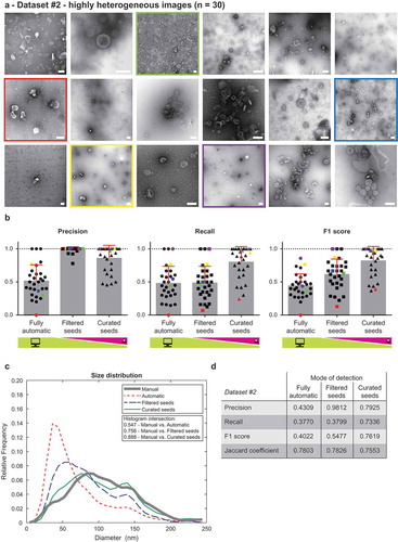
Figure 4. Comparison of the TEM ExosomeAnalyzer with other methods.
Representative TEM images used are shown in (a) for Patient 1 and in (b) for Patient 2, both samples are ovarian cancer ascites. The white bar represents 200 nm in each image. (c) Comparison of size distribution profiles of exs measured by TEM ExosomeAnalyzer (TEM EA), TRPS and NTA in the range applicable for all methods depicts coherent results for all approaches. Representative cryo-EM images used are shown in (d) for Patient 2, arrowheads indicate EVs. EVs containing the characteristic phospholipid bilayer (white arrowheads) as well as multi-layered vesicles (yellow arrowheads) and electron dense particles, which are likely lipoprotein particles (red arrows), were observed. (e) Comparison of size distribution profiles of EVs from Patient 2 measured by TEM ExosomeAnalyzer (TEM EA), TRPS, NTA and cryo-EM (data were acquired using TEM EA, each EV was manually outlined) in the range applicable for all methods depicts coherent results for all approaches. TEM EA provides comparable results to those of TRPS and NTA. Moreover, TEM EA and cryo-EM are able to analyse also vesicles smaller than the detection limit of TRPS and NTA. Interestingly, it seems that EVs do not shrink during processing for TEM as evidenced by largely overlapping histograms between TEM EA and cryo-EM.
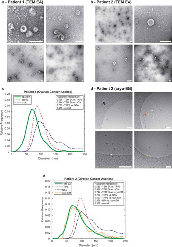
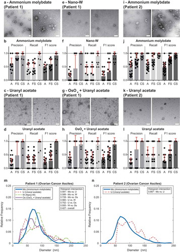
Figure 5. Performance of TEM ExosomeAnalyzer – different negative staining methods.
The performance of TEM ExosomeAnalyzer with respect to different negative staining protocols was performed. The white bar represents 200 nm in each image. Representative images and performance of the software in three modes (A – fully automatic, FS – filtered seeds, CS – curated seeds) are shown for EVs isolated from patient ovarian cancer ascites. Each symbol in the graphs corresponds to result for one image. Patient 1 ascites EVs were stained with ammonium molybdate (a and b), uranyl acetate (c and d), nano-W (e and f) and osmium tetroxide + uranyl acetate (g and h). Patient 2 ascites EVs were stained only by ammonium molybdate (i and j) and uranyl acetate (k and l). Comparison of size distribution profiles of EVs obtained by TEM ExosomeAnalyzer (in CS mode) using different staining techniques (m – patient 1, n – patient 2). High level of performance and similar size distribution profiles of EVs were achieved with all protocols tested.