Figures & data
Figure 1. Analyses of 10 individual fractions of MIA PaCa-2 sEVs separated by iodixanol density gradient centrifugation. An equal volume (15 µL) of fraction samples was loaded for western blotting (a) and silver staining (b) analyses. Particle concentrations (c) were estimated by NTA using NanoSight (n = 5). (d) Protein concentration was estimated by BCA assay (n = 2). The relative amount of protein was calculated based on the particle numbers and mode diameters (for volumes) estimated by NTA. (e) Particle diameter distribution profiles for Fr. 1 and Fr. 3 estimated by NTA. Black lines show the average histogram calculated from the data of five measurements, the plots of which are superimposed (thin coloured lines). Mode and mean (± SD) diameters for the average histogram are indicated. (f) Circles (red) and triangles (black) indicate mode and mean diameters estimated from each measurement, respectively. The mean values of the five measurements are represented as solid horizontal lines. Two-tailed unpaired t-test was used to evaluate statistical significance: # p < 0.05; ## p < 0.01.
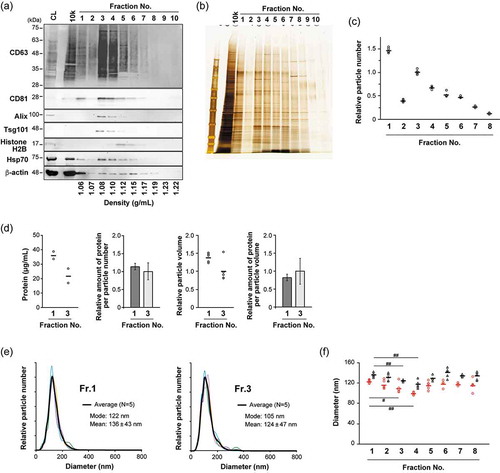
Figure 2. AFM analysis of fractionated MIA PaCa-2 sEVs. (a) AFM images obtained in PBS, indicated by colour changes corresponding to the height; colour bar: 70 nm. Scale bars, 500 nm. (b) Height and diameter histograms estimated by AFM. (c) The size distributions are presented as box plots (with median and quartiles). Whiskers in the box plots represent 1.5 times the interquartile range (IQR) or the highest or lowest point, whichever is shorter. The small circles represent outliers. X marks indicate the mean values. Vesicles with a height >15 nm were analyzed; Fr. 1: n = 125, Fr. 3: n = 174. Two-tailed unpaired t-test was used to evaluate statistical significance: * p < 0.001. The diameter was calculated from the object area under the assumption that the objects were round.
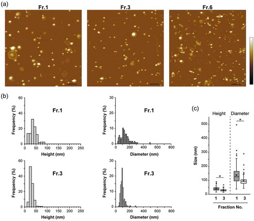
Figure 3. Distributions of zeta potentials of vesicles in Fr. 1 and Fr. 3 fractionated MIA PaCa-2 sEVs are shown by histograms (a) and box and whisker plots (b). Boxes represent the interquartile range (IQR) with median and whiskers extending to the extreme values within 1.5 times the IQR. A dot represents one outlier. X marks indicate the mean values. The zeta potentials were evaluated on an on-chip microcapillary electrophoresis system. Fr.1: n = 106, Fr.3: n = 69. Two-tailed unpaired t-test was used to evaluate statistical significance: * p < 0.001.
Table 1. The rate of vesicles bound with MFGE8-GNPs. The vesicles adsorbed on the substrates were counted using two independently prepared samples, and the total numbers are indicated.
Figure 4. Detection of PS on EV surfaces by gold labelling. MIA PaCa-2 sEVs were labelled using 20-nm GNPs conjugated with MFGE8 and imaged by AFM in air. Representative AFM images of MIA PaCa-2 Fr.1 (upper) and Fr.3 (lower). In the topographic (height) image, arrows and arrowheads indicate the vesicles unbound and bound with GNPs, respectively (left). GNPs were discerned by their regular round shape, height, and clear phase contrast (right). Scale bars: 200 nm, colour bars: 50 nm.
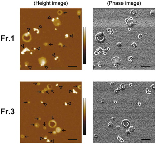
Figure 5. Thrombin generation assay for MIA PaCa-2 sEVs. Thrombin concentrations generated in the presence of an equal volume of fraction samples (left, n = 3). Relative thrombin production was calculated per particle number (centre) and per protein content (right).
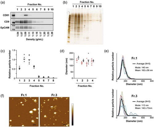
Figure 6. Analyses of 10 individual fractions of HT-29 sEVs separated by iodixanol density gradient centrifugation. Western blotting (a) and silver staining (b) analyses. Particle concentration (c) and diameters (d and e) were estimated by NTA (n = 5). (d) Circles (red) and triangles (black) indicate mode and mean diameters estimated from each measurement, respectively. The mean values of the five measurements are represented as solid horizontal lines. (e) In diameter distribution profiles for Fr.1 and Fr.3; black lines show the average histogram calculated from the data of five measurements, the plots of which are superimposed (thin coloured lines). Mode and mean (± s.d.) diameters for the average histogram are indicated. (f) AFM images for Fr.1 and Fr.3 obtained in PBS. Scale bars: 200 nm, colour bar: 100 nm.