International market exposure to sovereign ESG

Figures & data

Figure 1. Heatmap of Country ESG scores.

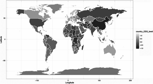
Figure 2. Descriptive plots of the ESG scores.

Notes: The panel on the left shows a boxplot of scores at the issue level. The panel on the right shows histograms, scatterplots and correlations of E, S & G pillar values across countries and years.

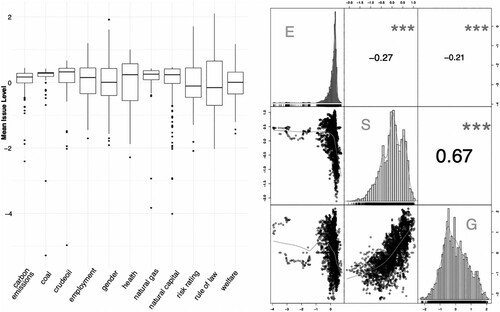
Figure 3. Baseline estimates and macroeconomic controls.

Notes: We plot the time-series of t-statistics in fixed-effect panel models (Equation (1(1) $r_{t+1,n}={\alpha }_{t+1,n}+\sum _{k=1}^K({\beta }_{t+1}^{(k)}{c}_{t,n}^{(k)}+{\eta }_t^{(k)}\mathrm{\Delta }{c}_{t,n}^{(k)})+{ϵ}_{t+1,n},$(1) )) run on 10 years of data, at the pillar level. The panel on the left shows the analysis for fixed income markets while the one on the right pertains to equity markets. The horizontal dashed lines mark the 99% threshold for the significance of the coefficients. The bottom set of plots include macroeconomic controls as defined in model (2(2) $r_{t+1,n}={\alpha }_{t+1,n}+\sum _{k=1}^K({\beta }_{t+1}^{(k)}{c}_{t,n}^{(k)}+{\eta }_t^{(k)}\mathrm{\Delta }{c}_{t,n}^{(k)})+\sum _{l=1}^L{\psi }_{t+1}^{(l)}\mathrm{\Delta }{m}_{t,n}^{(l)}+{ϵ}_{t+1,n},$(2) ).

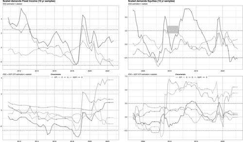
Figure 4. Analysis at issue level for equity & fixed income markets with macro variables.

Notes: We plot the time-series of t-statistics in fixed-effect panel models (Equation (2(2) $r_{t+1,n}={\alpha }_{t+1,n}+\sum _{k=1}^K({\beta }_{t+1}^{(k)}{c}_{t,n}^{(k)}+{\eta }_t^{(k)}\mathrm{\Delta }{c}_{t,n}^{(k)})+\sum _{l=1}^L{\psi }_{t+1}^{(l)}\mathrm{\Delta }{m}_{t,n}^{(l)}+{ϵ}_{t+1,n},$(2) )) estimated on 10 years of data, at the issue level. The panel on the top shows the analysis for equity markets while the one on the bottom pertains to fixed income markets. The horizontal dashed lines mark the 99% threshold for the significance of the coefficients.

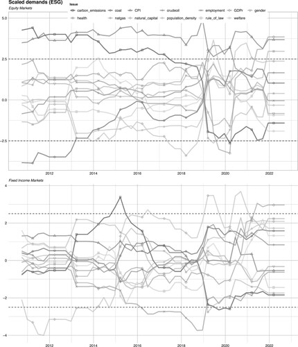
Figure 5. Latent demand distribution & $R^2$ for equity & fixed income markets with macro variables.

Notes: We plot the quantiles of the fixed effects in the panel models (Equation (2(2) $r_{t+1,n}={\alpha }_{t+1,n}+\sum _{k=1}^K({\beta }_{t+1}^{(k)}{c}_{t,n}^{(k)}+{\eta }_t^{(k)}\mathrm{\Delta }{c}_{t,n}^{(k)})+\sum _{l=1}^L{\psi }_{t+1}^{(l)}\mathrm{\Delta }{m}_{t,n}^{(l)}+{ϵ}_{t+1,n},$(2) )) estimated on 10 years of data, at the issue level. The left hand top plot pertains to fixed income markets, the left hand bottom plot relates to equity markets and the right hand plot displays the $R^2$ of the models over time.

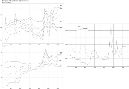
Table 1. Regression results for $\mathrm{\Delta }GDP$ fixed effects vs ESG scores.

Pillar	Term	Estimate	Std. Error	t-statistic	p-value	Confidence interval
2010–2018
ESG	(Intercept)	0.0336	0.0018	18.8313		[0.030,0.037]
ESG	esg_score	0.0061${}^{\ast }$	0.0033	1.8313	0.0672	[−0.000,0.013]
E	(Intercept)	0.0357	0.0015	24.0030		[0.033,0.039]
E	esg_score	0.0062${}^{\ast \ast \ast }$	0.0021	2.9250	0.0032	[0.002,0.010]
G	(Intercept)	0.0354	0.0018	19.9048		[0.032,0.039]
G	esg_score	−0.0001	0.0018	−0.0766	0.9391	[−0.004,0.003]
S	(Intercept)	0.0336	0.0022	15.3171		[0.029,0.038]
S	esg_score	0.0046	0.0043	1.0768	0.2880	[−0.004,0.013]
2019–2021
ESG	(Intercept)	0.1441	0.0071	20.3688		[0.130,0.158]
ESG	esg_score	0.0448${}^{\ast \ast \ast }$	0.0135	3.3092	0.0009	[0.018,0.071]
E	(Intercept)	0.1575	0.0058	27.0910		[0.146,0.169]
E	esg_score	−0.0051	0.0082	−0.6182	0.5288	[−0.021,0.011]
G	(Intercept)	0.1405	0.0071	19.8629		[0.127,0.154]
G	esg_score	0.0301${}^{\ast \ast \ast }$	0.0072	4.1551	0.0000	[0.016,0.044]
S	(Intercept)	0.1207	0.0089	13.5062		[1.103,1.138]
S	esg_score	0.0927${}^{\ast \ast \ast }$	0.0181	5.1151	0.0000	[0.057,0.128]

Notes: ${}^{\ast }p<$0.1; ${}^{\ast \ast }p<$0.05; ${}^{\ast \ast \ast }p<$0.01

Figure 6. Time-series of cumulative returns.

Notes: The strategy is given by Equation (6(6) ${\tilde{w}}_t^{(i)}=\underset{\mathrm{trend}\mathrm{signal}}{\underbrace{\sum _j\varphi \left({\alpha }_{t-1}^{i,j}\right)}}+\stackrel{\mathrm{ESGtilt}}{\overbrace{\kappa \cdot {\tilde{s}}_{t-1}^{(i)}}}+\underset{\mathrm{demand}\mathrm{component}}{\underbrace{\omega \cdot \sum _{l\in {\mathcal{D}}_t}{c}_{t-1,i}^{(l)}\cdot d_{t-1}^{(l)}}},$(6) ). Trading starts on 2011-01-03 and ends on 2021-02-05. Trend_Long_Short is the original strategy from Morgenstern, Coqueret, and Kelly (2021) (i.e. with $\omega =0$), while Trend_LS_plus_Demand pertains to the case $\omega =1/2$. The top plot provides cumulative returns, the middle plot provides daily returns and the bottom plot provides the drawdown profiles of the strategies.

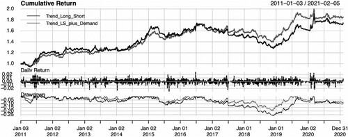
Table 2. Performance summary.

Strategy	Return	Risk	S.R.	VaR(5%)	Max DD	avg. D. length	T.E.
Trend L/S	$5.50\text{\%}$	$8.41\text{\%}$	0.65	$-0.85\text{\%}$	$26.69\text{\%}$	58.05	$0.00\text{\%}$
Trend L/S + Demand	$6.11\text{\%}$	$8.33\text{\%}$	0.73	$-0.84\text{\%}$	$19.42\text{\%}$	34.61	$5.74\text{\%}$

Notes: The strategy is given by Equation (6(6) ${\tilde{w}}_t^{(i)}=\underset{\mathrm{trend}\mathrm{signal}}{\underbrace{\sum _j\varphi \left({\alpha }_{t-1}^{i,j}\right)}}+\stackrel{\mathrm{ESGtilt}}{\overbrace{\kappa \cdot {\tilde{s}}_{t-1}^{(i)}}}+\underset{\mathrm{demand}\mathrm{component}}{\underbrace{\omega \cdot \sum _{l\in {\mathcal{D}}_t}{c}_{t-1,i}^{(l)}\cdot d_{t-1}^{(l)}}},$(6) ). Trading starts on 2011-01-03 and ends on 2021-02-05. The first line is the original strategy from Morgenstern, Coqueret, and Kelly (2021) (i.e. with $\omega =0$), while the second one pertains to the case $\omega =1/2$. The metrics are the average return, the volatility (standard deviation of returns), the Sharpe ratio, the Value-at-Risk, the maximum drawdown and the average drawdown length in days, and the tracking error with respect to the first strategy. All values are annualized.

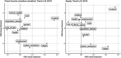
Figure 7. Sustainability demand versus sustainability score.

Notes: We locate both items in the plane for fixed income (left panel) and equity (right panel) components of the long-short trend following strategy of Section 5.1. The y-axis pertains to standard estimates from the baseline model of Equation (2(2) $r_{t+1,n}={\alpha }_{t+1,n}+\sum _{k=1}^K({\beta }_{t+1}^{(k)}{c}_{t,n}^{(k)}+{\eta }_t^{(k)}\mathrm{\Delta }{c}_{t,n}^{(k)})+\sum _{l=1}^L{\psi }_{t+1}^{(l)}\mathrm{\Delta }{m}_{t,n}^{(l)}+{ϵ}_{t+1,n},$(2) ). The x-axis is the weighted score of the strategy (each asset, via its country has a score which is aggregated at the portfolio level via its weight in the portfolio). The snapshot corresponds to December 2019. All components are sorted positively towards sustainability: a high crude oil score means low production and consumption of oil.

Morgenstern, C., G. Coqueret, and J. Kelly. 2021. “Tuning Trend-Following Strategies with Macro Esg Data.” The Journal of Impact and ESG Investing 2 (2): 117–136.

 Google Scholar