Effect of small water retention structures on diffusive CO₂ and CH₄ emissions along a highly impounded river

Figures & data

Figure 1. Location of (a) the Fluvià River catchment (northeastern Iberian Peninsula), with the position of the studied small water retention structures (SWRS; black circles, n = 11). See Table 1 for a detailed hydromorphological and physicochemical description of the waters impounded in the studied SWRS. (b) Scheme of a SWRS sampling unit (i.e., upstream free-flowing river, impounded water, and downstream free-flowing river) sampled at each study site.

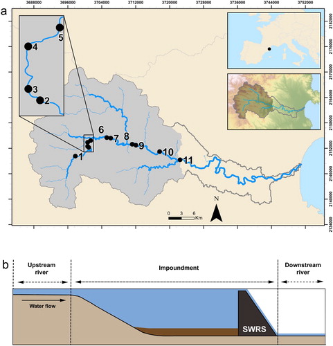
Table 1. Hydromorphological and physicochemical characteristics of the 11 studied impoundments. DOC = dissolved organic carbon, TDN = total dissolved nitrogen.

	Hydromorphological characteristics				Physicochemical characteristics
Impoundment	Surface area (ha)^a	Volume (hm^3)^a	Mean depth (m)^a	Water residence time (h)^b	Temperature (°C)^b	Conductivity (µS cm^-1)^b	DOC (mg L^-1)^b	TDN (mg L^-1)^b	Chlorophyll a (µg L^-1)^b
1	0.8	0.05	1.5	10.0 (6.9–13.2)	13.4 (7.8–18.4)	546 (480–623)	2.9 (2.1–4.0)	3.4 (1.4–4.8)	1.5 (1.0–2.1)
2	0.2	0.01	1.1	0.6 (0.4–0.9)	9.9 (5.8–19.3)	550 (477–622)	2.8 (1.7–3.3)	3.4 (1.5–5.1)	1.9 (0.3–3.4)
3	0.1	0.03	1.1	0.3 (0.2–0.4)	13.7 (6.7–20.3)	543 (472- 627)	2.2 (1.4–2.8)	3.6 (1.9–4.9)	2.1 (0.2–3.5)
4	0.2	0.03	1.3	1.3 (1.0–1.4)	14.9 (7.3–22.2)	751 (653–854)	2.2 (1.3–2.7)	3.8 (1.9–5.1)	3.3 (0.1–5.5)
5	0.3	0.02	1.3	1.5 (0.9–2.0)	14.5 (7.6–21.6)	725 (663–762)	2.4 (1.5–2.9)	3.6 (1.9–4.7)	2.1 (0.3–4.5)
6	0.2	0.02	0.8	0.6 (0.5–0.7)	15.9 (7.9–23.9)	813 (784–833)	2.1 (1.6–2.8)	3.0 (1.8–4.2)	1.8 (0.2–3.4)
7	0.2	0.03	0.7	0.8 (0.3–1.6)	17.2 (9.4–24.9)	882 (821–946)	2.1 (1.7–2.7)	2.9 (1.8–3.9)	2.3 (1.6–3.0)
8	1.9	0.04	1.8	10.0 (8.2–13.6)	21.2 (10.3–25)	933 (891–975)	2.0 (1.6–2.5)	2.8 (1.7–4.0)	4.0 (2.3–6.2)
9	1.6	0.02	1.3	4.3 (2.6–5.2)	16.7 (9.3–23.6)	1038 (915–1170)	2.5 (2.0–3.1)	1.6 (1.4–1.8)	21.9 (1.2–48.1)
10	2.7	0.01	0.6	3.2 (2.8–3.4)	12.9 (7.9–17.9)	682 (678–685)	2.0 (1.6–2.6)	2.3 (1.5–3.4)	6.1 (0.9–12.2)
11	9.6	0.12	0.7	40.8 (37.0–45.5)	13.2 (6.4–20.0)	575 (516–634)	2.4 (2.0–2.7)	2.1 (1.1–3.2)	11.4 (0.6–27.6)

^aMean of the 3 sampling dates. The temporal variation was negligible for these parameters

^bMean and range (in brackets) of the 3 sampling dates

Figure 2. Mean (a) CO₂ efflux, (b) CH₄ efflux and CH₄ efflux expressed as CO₂-equivalents (CO₂-equivalents = CO_2e; 1 g CH₄ = 28 g CO_2e; IPCC 2013), (c) partial pressure of CO₂ in water (), (d) partial pressure of CH₄ in water (), (e) gas transfer velocity of CO₂ (), and (f) gas transfer velocity of CH₄ () of the 11 SWRS grouped by sampling units (i.e., upstream river, impoundment water, and downstream river) during the 3 sampled seasons (i.e., spring, summer, and winter). Error bars represent standard error (SE). Significant differences of reported parameters between SWRS units (p < 0.05, Tukey’s post hoc test after repeated measures ANOVA) are marked with different letters above the bars.

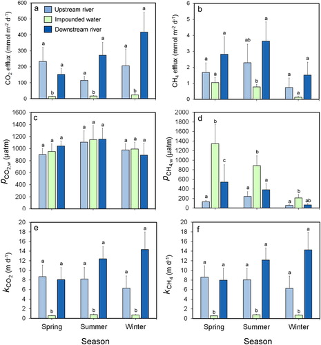
Figure 3. Downstream longitudinal patterns of the partial pressure of CO₂ in water () in (a) spring, (b) summer, and (c) winter and of the partial pressure of CH₄ in water () in (d) spring, (e) summer, and (f) winter across the 11 small water retention structure (SWRS) units (i.e., upstream river, impoundment water, and downstream river). The continuous solid lines represent the mean impoundment water or . Water flow direction goes from left to right.

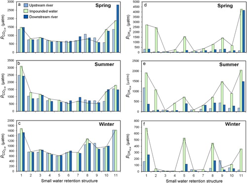
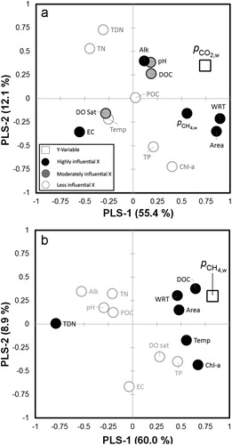
Figure 4. Loadings plot of the partial least squares (PLS) regression analysis for (a) partial pressure of CO₂ in water () and (b) partial pressure of CH₄ in water (). The graph shows how the Y-variable (squares) correlates with X-variables (circles) and the correlation structure. X-variables are classified according to their variable influence on projection value (VIP): highly influential (black circles), moderately influential (grey circles), and less influential (white circles). The X-variables situated near Y-variables are positively correlated to them and those situated on the opposite side are negatively correlated (see Supplemental Tables S1 and S2 for explanation of abbreviations and summary of PLS models, respectively).